Estimation of a vector-borne incubation period distribution: a Star Wars story

A mysterious disease has emerged on planet Naboo. Both infected humans and other extra-terrestrial life forms experience fever, severe headaches, skin rash and mild bleeding symptoms. The FIRST ORDER has sent health experts in the area. They identified the causing agent as being a vector-borne virus transmitted by an autochthonous mosquito species. Estimating the virus incubation period in vertebrate hosts would help to determine the duration of the containment measure to control the outbreak.

We will see here how to estimate an incubation period distribution in veterbrate hosts for a vector-borne pathogen. Vector-borne pathogens have a transmission cycle that involve invertebrate hosts (called the vector, i.e. mosquitoes, ticks, phlebotomes…) and vertebrate hosts (i.e., human or here extra-terrestrial :). We will assume that virus acquisition by the vertebrate host can only be due to an infectious mosquito bites. Incubation period (IP) is defined here as the time elapsed from virus acquisition to onset of symptoms in vertebrate host. We will only focus on symptomatic infection. Estimating the duration of IP in vertebrate hosts is not straightforward for vector-borne pathogens because date of infection through the bite of an infectious vector cannot usually be determined. People are usually bitten all the time by insects and they cannot trace back an infectious bite in time. We will exploit declared travel and symptom dates of travelers entering or leaving areas with ongoing virus transmission with interval-censored time to event (survival) analyses.

This code was used for the paper “Variability of Zika Virus Incubation Period in Humans” (https://www.ncbi.nlm.nih.gov/pubmed/30397624).

Load packages

You will need these packages.

library(msm)
library(survival)
library(plyr)
library(ggplot2)
library(lubridate)
library(interval)
library(icenReg)
#library(survminer) #Survminer is a nice package to visualize non-parametric survival curves. But I could'nt make it work on interval censored data.

Generate data

I generate a data.frame here. The first column of the data.frame is patient IDs, the second column indicates if they belong to the human race (Human=yes or no), the third column (Arrival) indicates the declared date of arrival in Naboo, the planet with active virus transmission. The last column indicates the duration of the stay in Naboo. All patients are travelers that visited the planet for a short period. There is no reported active virus transmission elsewhere in the galaxies. I generate a declared symptom onset date based on the date of arrival + a random number in the interval [1 ; Length_of_stay-1] + a incubation period drawn from a truncated (null or negative values not allowed) normal distribution, i.e. N(mean, SD=4). The mean for each patient category is indicated below.

set.seed(12)

Mean_ip_human <- 6 # Mean incubation period in human
Mean_ip_alien <- 12 # Mean incubation period in alien

data <- data.frame(ID=seq(1,194,1),
                      Name=c(paste("Wookie",1:14, sep="_"),paste("Ewok",1:50, sep="_"), paste("Stormtrooper",1:70, sep="_"), paste("Snowtrooper",1:60,sep="_")),
                      Human=c(rep("no",64), rep("yes",70+60)) ,
                      Arrival=sample(seq(as.Date("2016/01/01"), as.Date("2018/01/01"), by="day"), 194) ,
                      Length_of_stay_declared_days= round(rtnorm(194, mean = 15, sd = 4, lower=1)))

data<- ddply(data, .(ID), mutate,
                  Symptoms= if(Human=="no") {Arrival + sample(x = 1:(Length_of_stay_declared_days-1), 1) + round(rtnorm(1, mean = Mean_ip_alien, sd = 5, lower=1))}else{Arrival + sample(x = 1:(Length_of_stay_declared_days-1), 1) + round(rtnorm(1, mean = Mean_ip_human, sd = 5, lower=1))})

We use the lubridate package to convert dates:

data$Arrival <- ymd(as.character(data$Arrival)) #lubridate
data$Symptoms <- ymd(as.character(data$Symptoms )) #lubridate

Lets denote A for the date of Arrival in the zone of transmission (planet Naboo), D for date of Departure from planet Naboo and S for the date of Symptom declaration.

According to these terms we can calculate the following parameters:

• Duration of the stay in Naboo (Time_A_D)= D - A
• Duration from departure from Naboo and symptom onset (Time_D_S) = S - D
• Duration from arrival in Naboo and symptom onsets (Time_A_S) = S - A

We also use the lubridate package to calculate the day of departure from the day of arrival and the period of stay in the zone of active transmission.

data <- ddply(data, .(ID), mutate,
              Departure= Arrival + Length_of_stay_declared_days,
              Time_D_S= interval(Departure, Symptoms) %/% days(),
              Time_A_D= interval(Arrival,Departure ) %/% days(),
              Time_A_S= Time_A_D+Time_D_S)

data <- arrange(data, desc(Time_A_D))
data$ID <- factor(data$ID, levels=data$ID )

We can represent the travel data graphically:

p <- ggplot(data=data)
p <- p + geom_vline(xintercept = 0, color = "black", size=1 )
p <- p + geom_segment(aes(x = -Time_A_S , y = factor(ID), xend = -Time_D_S, yend = factor(ID), color=Human))
p <- p + geom_point(aes(x = -Time_A_S, y = factor(ID)), size = 2, color = "orange")
p <- p + geom_point(aes(x = -Time_D_S, y = factor(ID)), size = 2, color = "forestgreen")
p <- p + theme_bw(base_size = 20)
p <- p + theme(panel.grid.minor = element_blank(), panel.grid.major = element_blank(), axis.text.y=element_blank(), axis.ticks.y=element_blank())
#p <- p + facet_wrap(~Human, scales = "free_y", nrow=2)
p <- p + ggtitle("") + ylab("Individuals")
p <- p + scale_color_manual(values = c("dodgerblue3", "deeppink2"))
p <- p + scale_x_continuous(name="Time (days)", limits=c(-100,30), breaks=seq(-100,30,10))
p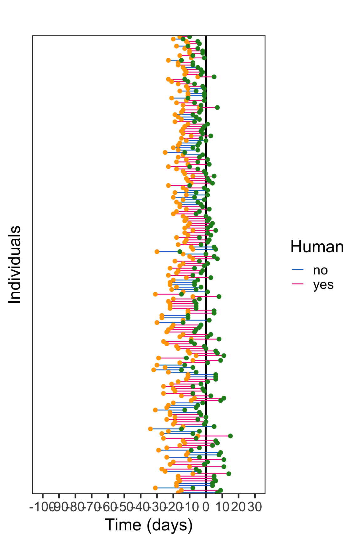

The vertical black line represents the onset of symptoms. Travel data from human and not human patients are represented with colored horizontal lines. The arrival and departure from the area with ongoing virus transmission is represented with an orange and green dot, respectively.

The exposure interval is delineated by the arrival date and the departure date for travelers that experienced symptoms after returning from travel, whereas the period separating the arrival date and the symptom onset date delineated the exposure interval in travelers experiencing illness during the journey.

We can thus define the exposure interval with 2 different manners. Concerning patients experiencing symptoms after departure from endemic zone: exposure interval = Time_A_D Concerning patients experiencing symptoms during the trip: exposure interval = Time_A_S

I am creating the interval censored data (Surv object) conditionally:

data$left <- NA
data$right <- data$Time_A_S

for(i in 1:nrow(data)) {
if(data[i,"Time_D_S"] < 0) {data[i,"left"] <- 0}else{data[i,"left"] <- data[i,"Time_D_S"]}
}

temp <- with(data, Surv(left,right,type="interval2"))

#Non-parametric model

I first use non-parametric time to event model, which are the most robust (no bias related to mispecification of the hazard distribution). I am using here the icfit function from the interval package.

fit<-icfit(temp~Human, data=data, conf.int=T )
#summary(fit)

#Cumulative distribution function
plot(fit, conf.int = F, COL = c("deeppink2","dodgerblue3"))
abline(h=0.5, col="gold3")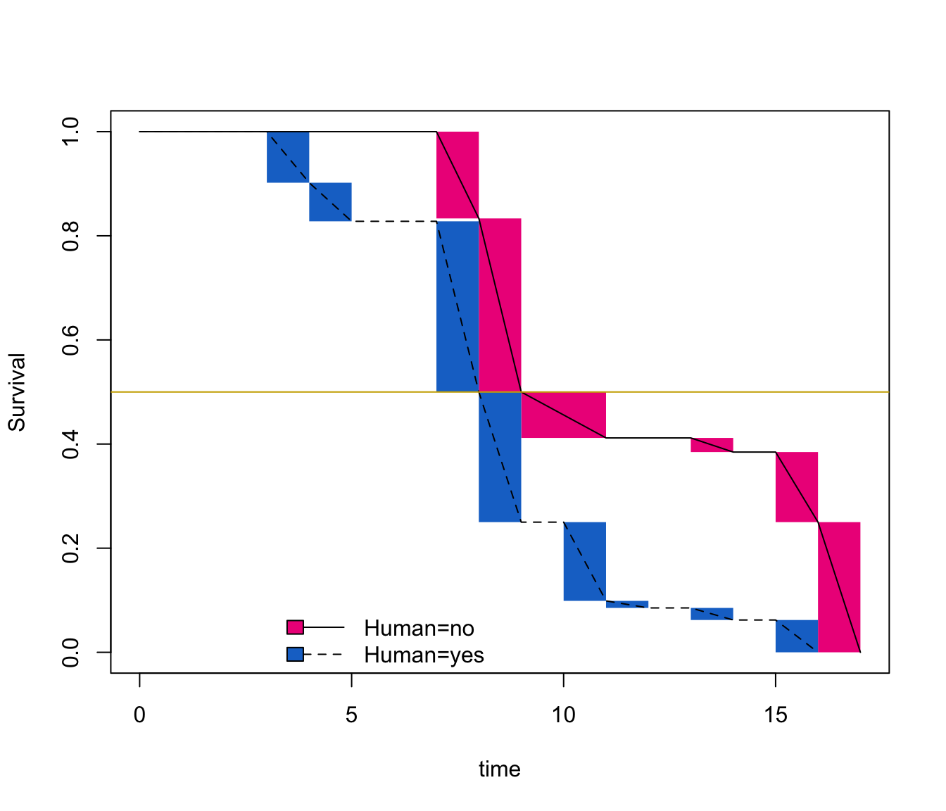

Summary(fit) provides non-parametric maximum likelihood estimates (NPMLEs) of the IP distribution (generalization of the Kaplan-Meier estimate) with a modified bootstrap confidence interval (CI) method. Estimates are calculated over a set of time intervals called Turnbull intervals, which represent the innermost intervals over a group of individuals in which NPMLE can change. Median survival estimates correspond to the time where the survival probability reaches 0.5 (gold horizontal line).

The median IP occured during the interval [6;7] for humans and [11;12] for extra-terrestrials. That correspond to mean values that we have setted up previously 😃.

We can apply some statistical tests (non-parametric log-rank tests) implemented in the interval package:

#logrank: Sun's scores
test<-ictest(temp~Human, data=data)
test

#logrank: Finkelstein's scores
test<-ictest(temp~Human, data=data, scores="logrank2")
test

#Wilcoxon-type tests
test<-ictest(temp~Human, data=data, scores="wmw")
test

#Wilcoxon-type tests, exact Monte Carlo
test<-ictest(temp~Human, data=data, scores="wmw", exact=T)
test

Patient category is significantly impacting the duration of virus incubation.

#Parametric model (accelerated failure-time regression model (AFT))

We now are going to model the incubation period distribution using parametric models (accelerated failure-time regression models (AFT).

Fully parametric models provide more efficient inference and quantification of uncertainty of time to event estimates (smoother probability distribution with restricted confidence intervals) at the cost of requiring a correct assumption of the baseline distribution family. The use of fully parametric models is also convenient because they link a time post virus exposure to a probability of symptom onset through an equation with estimated parameters.

We first have to determine the baseline function.

diag_baseline(temp ~ 1,
              model = "ph",
              data = data,
              dists = c("exponential", "weibull","loglogistic", "gamma", "lnorm"),
              lgdLocation = "topright")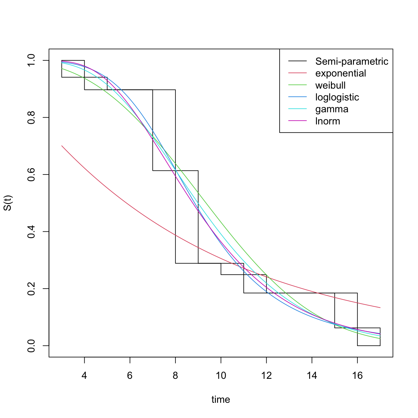

I choose the loglogistic baseline distribution. We will now use the icenReg package (https://cran.r-project.org/web/packages/icenReg/vignettes/icenReg.pdf).

fit_loglogistic <- ic_par(temp ~ Human, data = data, model = "aft", dist = "loglogistic")
summary(fit_loglogistic)

newdata<-data.frame(Human=levels(factor(data$Human)))
rownames(newdata) <- c("Not human", "Human")

survCIs(fit_loglogistic, p=0.5, newdata = newdata) #Median estimates
survCIs(fit_loglogistic, p=0.95, newdata = newdata) #95th centiles estimates

plot(fit_loglogistic, newdata = newdata, fun = "cdf")
abline(h=0.5, col="gold3")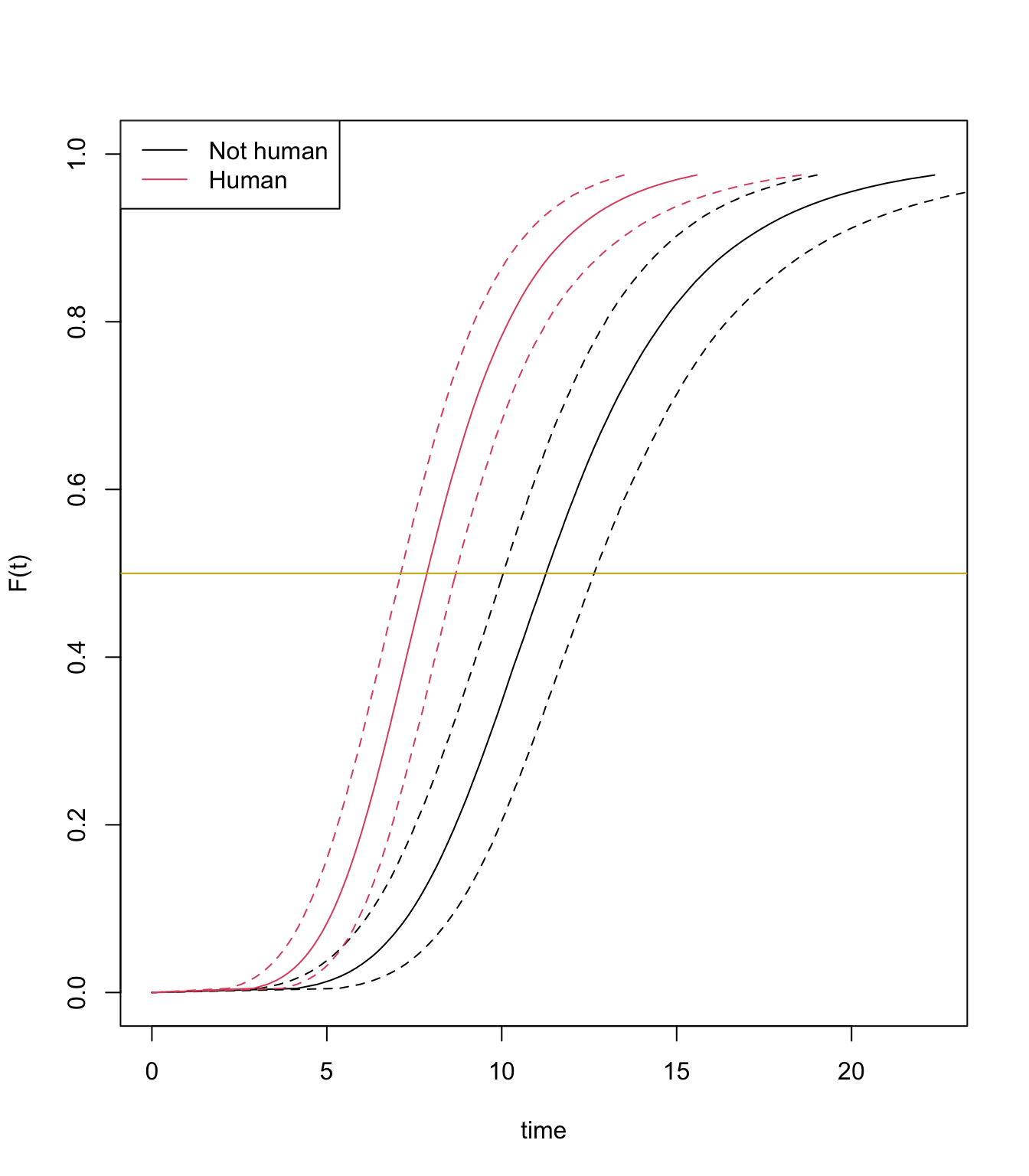

The plot displays parametric estimates of virus incubation period probabilities over time.

The median estimates are 11.2 days and 6.4 days for aliens and human, respectively.

#Bayesian accelerated failure-time regression model (AFT):

The icenReg R package dedicated to interval censored data offers the opportunity to extend fully parametric models to the Bayesian framework. In this case, Bayesian inference is used to estimate the log-logistic baseline distribution parameters (shape and scale) instead of maximum likelihood estimation (MLE).

We will use flat priors here. You can refer to icenReg package documentation if you want to use priors.

bayes_fit <- ic_bayes(temp ~ Human,
                      data = data,
                      model = "aft", dist = "loglogistic",
                      controls = bayesControls(samples = 100000, chains = 4, useMLE_start = TRUE,
                                               burnIn = 1000))

(CI <- survCIs(bayes_fit, p=0.5, newdata = newdata))
(CI2 <- survCIs(bayes_fit, p=0.95, newdata = newdata))

plot(bayes_fit, newdata = newdata, fun = "cdf")
abline(h=0.5, col="gold3")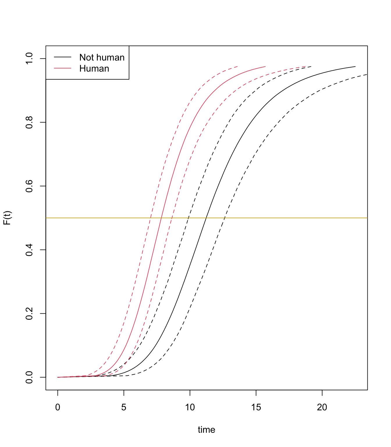

The Bayesian median estimates are 11.12 days and 6.39 days for aliens and human, respectively, it is not very different from AFT estimates.