Methods to estimate intra-mosquito systemic infection dynamics: a Star Wars story
Background
Aedes gunganiensis, a mosquito species native of Naboo planet, was suspected to be the main vector of the mysterious virus that has emerged on planet Naboo (NabooV) (refer to the previous part). However, the extent of trades among planets from different galaxies at Class 2 hyperdrive has favored the invasion of new mosquito species. Ochlerotatus dagobahus has first invaded the swamps and wetlands of Naboo before to adapted to more urban environments on the planet. Health experts from the FIRST ORDER are conducting experiments to assess intra-mosquito virus dynamics in these species.
We will see here how to estimate biologically relevant parameters from cumulative proportions of infected mosquito with a disseminated virus infection that have been experimentally exposed to the virus.
This code was used for the paper “Epidemiological significance of dengue virus genetic variation in mosquito infection dynamics” (https://www.ncbi.nlm.nih.gov/pubmed/30005085) and “The native European Aedes geniculatus mosquito species can transmit Chikungunya virus” (https://www.ncbi.nlm.nih.gov/pubmed/31259662)
Import data
#Import data:
data <- read.table("VC_data.txt", h=T, stringsAsFactors=T )
head(data)
## Mosquito_species dpi Virus_Body Virus_Head
## 1 Aedes_gunganiensis 4 1 0
## 2 Aedes_gunganiensis 4 1 0
## 3 Aedes_gunganiensis 4 1 0
## 4 Aedes_gunganiensis 4 1 0
## 5 Aedes_gunganiensis 4 1 0
## 6 Aedes_gunganiensis 4 1 0str(data)## 'data.frame': 406 obs. of 4 variables:
## $ Mosquito_species: Factor w/ 2 levels "Aedes_gunganiensis",..: 1 1 1 1 1 1 1 1 1 1 ...
## $ dpi : int 4 4 4 4 4 4 4 4 4 4 ...
## $ Virus_Body : int 1 1 1 1 1 1 1 0 0 1 ...
## $ Virus_Head : int 0 0 0 0 0 0 0 0 0 0 ...Here are how the data set looks like.
Mosquito_species: Either Aedes_gunganiensis or Ochlerotatus_dagobahus. dpi: day post virus exposure (/infection). Virus_Body: Body infection status. 1 for infected and 0 for non-infected. Virus_Head: Head infection status that is used as a proxy for systemic infection. 1 for infected and 0 for non-infected.
After a given time post experimental virus exposure, mosquitoes were sacrificed and scored for the presence of virus in their heads and bodies. Presence of virus in bodies indicates a midgut infection, while presence of virus in heads indicates a systemic (disseminated) infection.
We will focus here on systemic infection prevalences, that is, the proportion of mosquito with a disseminated virus infection at each time point post virus exposure. We thus now select mosquitoes with a body infection.
data_dissem <- subset(data, Virus_Body==1)We now calculate systemic infection prevalences with 95% CI.
Calculate systemic infection prevalences
ob.diss <- ddply(data_dissem, .(Mosquito_species, dpi),summarise, N= length(Virus_Head), Pos=sum(Virus_Head), Prev= sum(Virus_Head)/length(Virus_Head), low=prop.test(sum(Virus_Head),length(Virus_Head))$conf.int[1],
      upper=prop.test(sum(Virus_Head),length(Virus_Head))$conf.int[2])

ob.diss
## Mosquito_species dpi N Pos Prev low upper
## 1 Aedes_gunganiensis 4 28 3 0.10714286 0.028087469 0.2937003
## 2 Aedes_gunganiensis 6 29 19 0.65517241 0.456638554 0.8140244
## 3 Aedes_gunganiensis 8 18 12 0.66666667 0.411547974 0.8564334
## 4 Aedes_gunganiensis 12 19 15 0.78947368 0.539020276 0.9302931
## 5 Aedes_gunganiensis 15 35 26 0.74285714 0.564299668 0.8689425
## 6 Aedes_gunganiensis 18 31 24 0.77419355 0.584591818 0.8972206
## 7 Aedes_gunganiensis 21 30 23 0.76666667 0.572997657 0.8936498
## 8 Ochlerotatus_dagobahus 4 31 1 0.03225806 0.001686181 0.1851058
## 9 Ochlerotatus_dagobahus 6 26 2 0.07692308 0.013436626 0.2659973
## 10 Ochlerotatus_dagobahus 8 19 3 0.15789474 0.041696730 0.4049326
## 11 Ochlerotatus_dagobahus 12 25 15 0.60000000 0.388903024 0.7818808
## 12 Ochlerotatus_dagobahus 15 32 29 0.90625000 0.738334455 0.9754703
## 13 Ochlerotatus_dagobahus 18 37 37 1.00000000 0.882869683 1.0000000
## 14 Ochlerotatus_dagobahus 21 25 25 1.00000000 0.834226993 1.0000000Visual representation with ggplot2
# plot curve

#Create a custom color scale (each Mosquito_species level will be linked to a color)
library(RColorBrewer)
myColors <- brewer.pal(8,"Dark2")
names(myColors) <- levels(ob.diss$Mosquito_species)
colScale <- scale_colour_manual(name = "Mosquito_species",values = myColors)


#Visualization:
require("grid")
## Le chargement a nécessité le package : gridp <- ggplot()
p <- p + geom_point(data=ob.diss, aes(x = dpi, y = Prev, color=Mosquito_species, size=N))
p <- p + theme_bw(base_size =20)
p <- p + geom_point(data=ob.diss, aes(x=dpi, y=low,color=Mosquito_species), shape=95, size=3 )
p <- p + geom_point(data=ob.diss, aes(x=dpi, y=upper,color=Mosquito_species), shape=95, size=3 )
p <- p + facet_wrap(~Mosquito_species, scales = "free_y")
p <- p + ylab("NabooV systemic infection (%)") + xlab(label="Days post-exposure")
p <- p + colScale
p <- p + ylim(0, 1.09)
p <- p + guides(colour=FALSE)
p <- p + theme(axis.title.x=element_text(size=20, color="black", vjust=-1), axis.title.y=element_text(size=20, color="black", vjust=1, margin=margin(0,20,0,0)))
p <- p + theme(plot.margin = unit(c(2,2,2,2), "lines"))
print(p)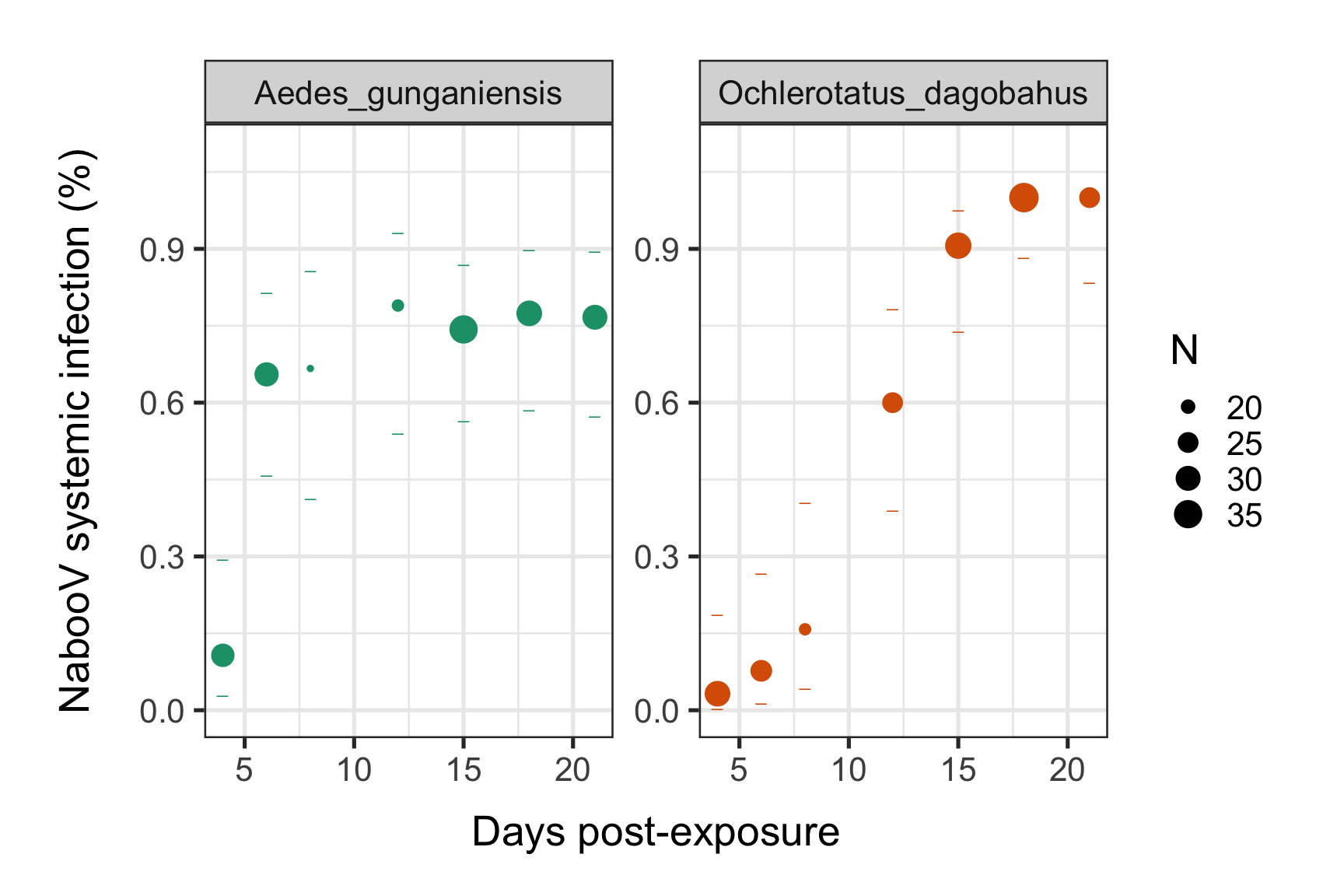
#Save in pdf:
#ggsave(filename = "Systemic_infection_dynamics.pdf", p,width = 16,height = 10)

#Save in svg:
#svglite("Systemic_infection_dynamics.svg", width = 16,height = 10)
#print(p)
#dev.off()
We can see an increase of the NabooV systemic infection prevalences post experimental virus exposure over time until to reach a saturation level (plateau). This saturation level seems to be lower (around 75%) for Ae. gunganiensis as compared to 100% for Och. dagobahus. But the time need by the NabooV to reach this plateau is faster for Ae. gunganiensis. We now want to get biological meaningful estimates that describe these intra-mosquitoes systemic infection dynamics.
Method 1: Nonlinear regression estimates with the “drm” function from the “drc”" R package.
#Fit a 3 parameters logistic model (L.3) to data using the "drm" function from the "drc"" R package.
modelex <- drm(Prev ~ dpi,Mosquito_species, weights = 1/N, data = ob.diss, fct = L.3())
summary(modelex)
##
## Model fitted: Logistic (ED50 as parameter) with lower limit fixed at 0 (3 parms)
##
## Parameter estimates:
##
## Estimate Std. Error t-value p-value
## b:Aedes_gunganiensis -1.501494 0.412564 -3.6394 0.006594 **
## b:Ochlerotatus_dagobahus -0.517568 0.067613 -7.6549 5.990e-05 ***
## d:Aedes_gunganiensis 0.744954 0.020901 35.6418 4.205e-10 ***
## d:Ochlerotatus_dagobahus 1.017594 0.040567 25.0840 6.828e-09 ***
## e:Aedes_gunganiensis 4.995885 0.220533 22.6537 1.527e-08 ***
## e:Ochlerotatus_dagobahus 11.245550 0.356767 31.5207 1.117e-09 ***
## ---
## Signif. codes: 0 '***' 0.001 '**' 0.01 '*' 0.05 '.' 0.1 ' ' 1
##
## Residual standard error:
##
## 0.001825472 (8 degrees of freedom)We get 3 estimated parameters (b,d and e) for each species. Let renames them as K, B and M.
The probability of systemic infection at a given time point (t) is governed by K: the saturation level (the maximum proportion of mosquitoes with a systemic infection), B: the slope factor (the maximum value of the slope during the exponential phase of the cumulative function, scaled by K) and M: the lag time (the time at which the absolute increase in cumulative proportion is maximal).
#Create a data.frame with all parameter estimates (d, b, e are replaced by K, B, M labels). As the 3 parameters logistic model estimates -B, the opposite (true slope) was selected here :
parameters <- data.frame(K=coef(modelex)[grep("d:", names(coef(modelex)))], B=-coef(modelex)[grep("b:", names(coef(modelex)))], M=coef(modelex)[grep("e:", names(coef(modelex)))] )
rownames(parameters) <- str_replace(rownames(parameters), "d:", "")

kable(parameters)| K | B | M | |
|---|---|---|---|
| Aedes_gunganiensis | 0.7449544 | 1.5014945 | 4.995885 |
| Ochlerotatus_dagobahus | 1.0175938 | 0.5175684 | 11.245549 |
#write.table(parameters, "Estimated_param.txt", quote = F, row.names = F)We add predicted values on the graph. We will use the expand.grid function to generate a data frame with 100 lines per time points, for a range of time points going from 0 to 26 days post infection for each species. We will then generate predicted values of systemic infection proportions in a new column for each combination.
# Creation of a new data.frame with dpi values ranging from 1 to 20 with 100 steps.
newdata <- expand.grid(dpi=seq(0,26, length=100), Mosquito_species=unique(ob.diss$Mosquito_species), N=NA)
# Prevalence predictions with confidence intervals
pm <- predict(modelex, newdata=newdata, interval="confidence")
# New data with predictions
newdata$p <- pm[,1]
newdata$pmin <- pm[,2]
newdata$pmax <- pm[,3]
# plot curve

p <- p + geom_line(data=newdata, aes(x=dpi, y=p, color=Mosquito_species))
print(p)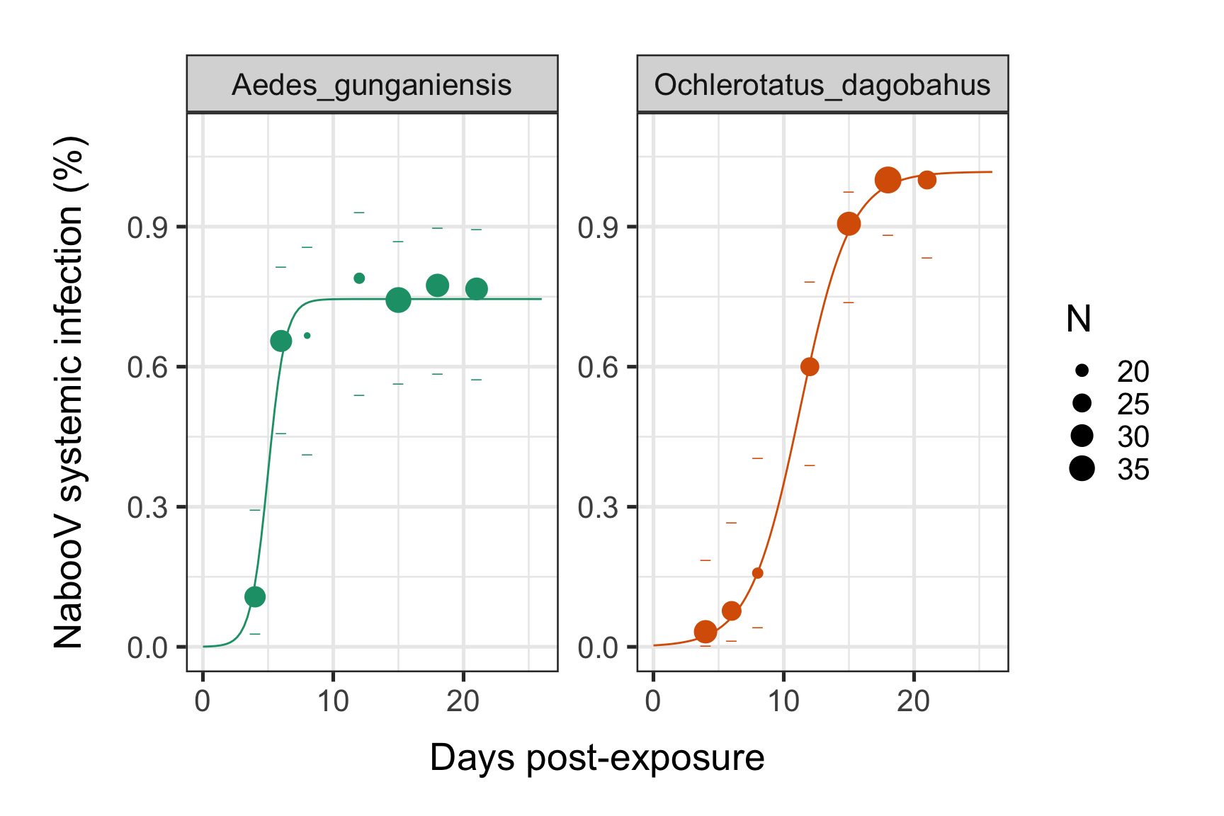
Without the facet_wrap pannels:
#Visualization:
require("grid")
p1 <- ggplot()
p1 <- p1 + geom_point(data=ob.diss, aes(x = dpi, y = Prev, color=Mosquito_species, size=N))
p1 <- p1 + theme_bw(base_size =20)
p1 <- p1 + geom_point(data=ob.diss, aes(x=dpi, y=low,color=Mosquito_species), shape=95, size=3 )
p1 <- p1 + geom_point(data=ob.diss, aes(x=dpi, y=upper,color=Mosquito_species), shape=95, size=3 )
p1 <- p1 + ylab("NabooV systemic infection (%)") + xlab(label="Days post-exposure")
p1 <- p1 + colScale
p1 <- p1 + ylim(0, 1.09)
p1 <- p1 + guides(colour=FALSE)
p1 <- p1 + geom_line(data=newdata, aes(x=dpi, y=p, color=Mosquito_species))
p1 <- p1 + theme(axis.title.x=element_text(size=20, color="black", vjust=-1), axis.title.y=element_text(size=20, color="black", vjust=1, margin=margin(0,20,0,0)))
p1 <- p1 + theme(plot.margin = unit(c(2,2,2,2), "lines"))
print(p1)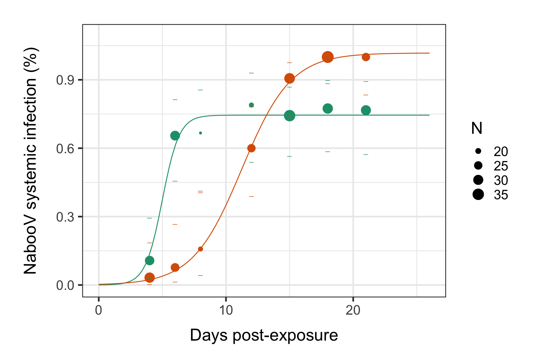
The “drc”" R package make it easy to estimate times (in days) to reach a given proportion of systemic infection for each species, eg. DT-5%, DT-50%, and DT-90% where 95% confidence intervals are obtained using the delta method.
ED(modelex, c(5, 50, 90), interval = "delta")##
## Estimated effective doses
##
## Estimate Std. Error Lower Upper
## e:Aedes_gunganiensis:5 3.03488 0.52512 1.82396 4.24580
## e:Aedes_gunganiensis:50 4.99588 0.22053 4.48734 5.50443
## e:Aedes_gunganiensis:90 6.45924 0.50743 5.28911 7.62937
## e:Ochlerotatus_dagobahus:5 5.55656 0.68575 3.97522 7.13791
## e:Ochlerotatus_dagobahus:50 11.24555 0.35677 10.42284 12.06826
## e:Ochlerotatus_dagobahus:90 15.49083 0.76881 13.71796 17.26371The growth rate (B) can be transformed into Δt which correspond to the rise time of the exponential function (time taken for a virus to rise from 10% to 90% of its saturation level) with the formula: log(81)/B [http://condellpark.com/kd/sars_files/LogisticRisetime.pdf]
parameters$deltaT <- log(81)/parameters$B
kable(parameters)| K | B | M | deltaT | |
|---|---|---|---|---|
| Aedes_gunganiensis | 0.7449544 | 1.5014945 | 4.995885 | 2.926717 |
| Ochlerotatus_dagobahus | 1.0175938 | 0.5175684 | 11.245549 | 8.490567 |
#write.table(parameters, "Estimated_param.txt", quote = F, row.names = F)Method 2: Maximum likelihood estimates
This code was developed by Robert C. Reiner, Jr, Assistant Professor of Health Metric Sciences at the University of Washington (http://rcreinerjr.com). I just tweaked it a little to adapt it to my way of coding.
By the way, I would say that my coding style is stuck somewhere between the base R language and the tidyverse (ie. plyr)). There are several tracks to go to the same spot and you might find better ones!
Based on the 3- parameters logistic model: f(t,(K,B,M)) = K / (1+exp(-B * (t - M))), this method provides the best estimates of the three parameters to maximize the global likelihood function (i.e., the sum of binomial probabilities at each time point post virus exposure) and accounts for differences in sample size when estimating parameters values.
You will need these function to make it work.
#The 3 parameter function:
Transform <- function(datvec, parvec){
    K <- parvec[1]
    B <- parvec[2]
    M <- parvec[3]
    return(K / (1+exp(-B * (datvec - M))))
}

#Idem but with the 3 parameters specified (it will be used for visualisation purpose)
Transform_b <- function(datvec, K, B, M){
    return(K / (1+exp(-B * (datvec - M))))
}

#Initial guess of the parameters to be optimized over by the subplex function.
InitialGuess <- runif(3)

#Likelihood function to be optimized by the subplex function. This function takes 2 arguments: (i) a vector of three random value that would be optimized and (ii) the raw systemic infection data (ie, data_dissem object obtained above).
#This function determine a global likelihood function based on the sum of binomial probabilities at each time point post virus exposure. It will be feeded to the subplex function to obtained the best parameters estimates for each mosquito species.

vec <- runif(3)

LL <- function(vec,tmpData){
    tmpData$tmp <- Transform(tmpData$dpi, vec)
    tmpDay <- sort(unique(tmpData$dpi))
    tmpVir <- unique(tmpData$Mosquito_species)
    tmpPos <- tmpSamp <- tmpProb <- matrix(NA,length(tmpVir),length(tmpDay))
    for (v in 1:length(tmpVir)){
        for (i in 1:length(tmpDay)){
            tmploc <- which(tmpData$dpi == tmpDay[i] & tmpData$Mosquito_species == tmpVir[v])
            tmpSamp[v,i] <- length(tmploc)
            tmpPos[v,i] <- length(which(tmpData$Virus_Head[tmploc]==1))
            tmpProb[v,i] <- tmpData$tmp[tmploc[1]]
        }
    }
    tmpSamp <- as.vector(tmpSamp)
    tmpPos <- as.vector(tmpPos)
    tmpProb <- as.vector(tmpProb)
    if (min(tmpProb)<=0 | max(tmpProb)>=1 | vec[1] > 1 | vec[1] < 0){
        return(-1e8)
    } else {
        return(sum(dbinom(tmpPos,tmpSamp,prob=tmpProb,log=TRUE)))
    }
}

#Inverse of the previous function. Because the subplex function minimize and not maximize a function.

NegLL <- function(vec,tmpData) return(-LL(vec,tmpData))

models <- dlply(data_dissem, "Mosquito_species", purrr::possibly(function(data_dissem) subplex(InitialGuess, NegLL, tmpData = data_dissem, control = list(maxit = 2000)), otherwise = NULL, quiet = TRUE ))

parameters_m2 <- do.call(rbind,lapply(models, '[[', 1))
parameters_m2 <- as.data.frame(parameters_m2)
colnames(parameters_m2) <- c("K", "B", "M")
parameters_m2$Mosquito_species <- row.names(parameters_m2)
#Dataframe with the parameter estimates for each Mosquito_species:
kable(parameters_m2)| K | B | M | Mosquito_species | |
|---|---|---|---|---|
| Aedes_gunganiensis | 0.7530613 | 1.8185820 | 4.982391 | Aedes_gunganiensis |
| Ochlerotatus_dagobahus | 1.0000000 | 0.5588679 | 10.883230 | Ochlerotatus_dagobahus |
#The slope factor B can be transformed into deltaT, which correspond to the time required to rise from 10% to 90% of the saturation level:
parameters_m2$deltaT <- log(81)/parameters_m2$B
kable(parameters_m2)| K | B | M | Mosquito_species | deltaT | |
|---|---|---|---|---|---|
| Aedes_gunganiensis | 0.7530613 | 1.8185820 | 4.982391 | Aedes_gunganiensis | 2.416415 |
| Ochlerotatus_dagobahus | 1.0000000 | 0.5588679 | 10.883230 | Ochlerotatus_dagobahus | 7.863127 |
Estimates are slightly different from those from method 1 (non-linear regression).
Visual representation with ggplot2:
# Creation of a new dataframe with dpi values ranging from 1 to 20 with 100 steps.
newdata <- expand.grid(dpi=seq(0,26, length=100), Mosquito_species=unique(ob.diss$Mosquito_species), N=NA)
# Generate data from regression
newdata <- merge(newdata, parameters_m2,by.x="Mosquito_species", by.y="Mosquito_species")
newdata$prevalence <- with(newdata, Transform_b(dpi, K, B, M))


# plot curve

#Create a custom color scale (each Mosquito_species level will be linked to a color)
library(RColorBrewer)
myColors <- brewer.pal(8,"Dark2")
names(myColors) <- levels(ob.diss$Mosquito_species)
colScale <- scale_colour_manual(name = "Mosquito_species",values = myColors)


#Visualization:
require("grid")
p <- ggplot()
p <- p + geom_point(data=ob.diss, aes(x = dpi, y = Prev, color=Mosquito_species, size=N))
p <- p + theme_bw(base_size =20)
#p <- p + geom_ribbon(data=newdata, aes(x=dpi, y=p, ymin=pmin, ymax=pmax, fill=Mosquito_species), alpha=0.1, colour="white")
p <- p + geom_point(data=ob.diss, aes(x=dpi, y=low,color=Mosquito_species), shape=95, size=3 )
p <- p + geom_point(data=ob.diss, aes(x=dpi, y=upper,color=Mosquito_species), shape=95, size=3 )
p <- p + geom_line(data=newdata, aes(x=dpi, y=prevalence, color=Mosquito_species))
p <- p + facet_wrap(~Mosquito_species, scales = "free_y")
p <- p + ylab("DENV systemic infection (%)") + xlab(label="Days post-exposure")
p <- p + colScale
p <- p + ylim(0, 1.05)
p <- p + guides(colour=FALSE)
p <- p + theme(axis.title.x=element_text(size=20, color="black", vjust=-1), axis.title.y=element_text(size=20, color="black", vjust=1, margin=margin(0,20,0,0)))
p <- p + theme(plot.margin = unit(c(2,2,2,2), "lines"))
print(p)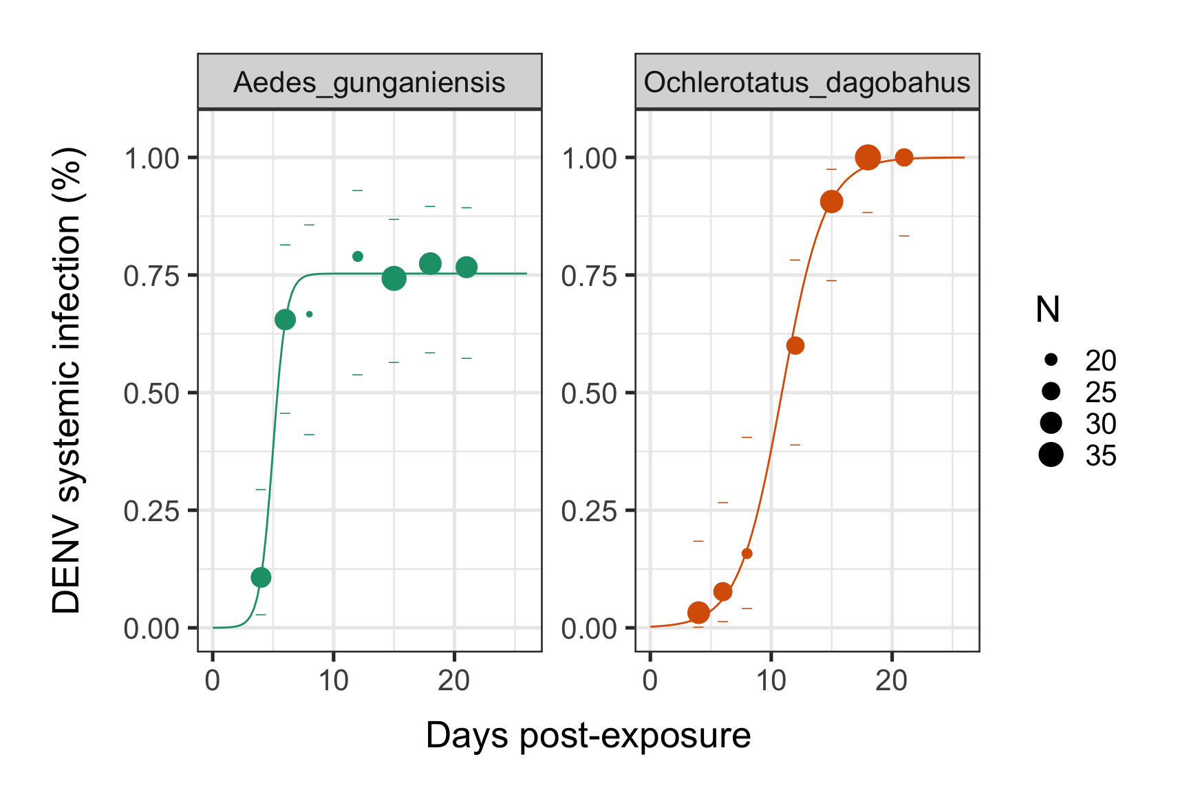
#Save in pdf:
#ggsave(filename = "Systemic_infection_dynamics.pdf", p,width = 16,height = 10)

#Save in svg:
#svglite("Systemic_infection_dynamics.svg", width = 16,height = 10)
#print(p)
#dev.off()
Without the facet_wrap
# Creation of a new dataframe with dpi values ranging from 1 to 20 with 100 steps.
newdata <- expand.grid(dpi=seq(0,26, length=100), Mosquito_species=unique(ob.diss$Mosquito_species), N=NA)
# Generate data from regression
newdata <- merge(newdata, parameters_m2,by.x="Mosquito_species", by.y="Mosquito_species")
newdata$prevalence <- with(newdata, Transform_b(dpi, K, B, M))


# plot curve

#Create a custom color scale (each Mosquito_species level will be linked to a color)
library(RColorBrewer)
myColors <- brewer.pal(8,"Dark2")
names(myColors) <- levels(ob.diss$Mosquito_species)
colScale <- scale_colour_manual(name = "Mosquito_species",values = myColors)


#Visualization:
require("grid")
p <- ggplot()
p <- p + geom_point(data=ob.diss, aes(x = dpi, y = Prev, color=Mosquito_species, size=N))
p <- p + theme_bw(base_size =20)
#p <- p + geom_ribbon(data=newdata, aes(x=dpi, y=p, ymin=pmin, ymax=pmax, fill=Mosquito_species), alpha=0.1, colour="white")
p <- p + geom_point(data=ob.diss, aes(x=dpi, y=low,color=Mosquito_species), shape=95, size=3 )
p <- p + geom_point(data=ob.diss, aes(x=dpi, y=upper,color=Mosquito_species), shape=95, size=3 )
p <- p + geom_line(data=newdata, aes(x=dpi, y=prevalence, color=Mosquito_species))
#p <- p + facet_wrap(~Mosquito_species, scales = "free_y")
p <- p + ylab("DENV systemic infection (%)") + xlab(label="Days post-exposure")
p <- p + colScale
p <- p + ylim(0, 1.05)
p <- p + guides(colour=FALSE)
p <- p + theme(axis.title.x=element_text(size=20, color="black", vjust=-1), axis.title.y=element_text(size=20, color="black", vjust=1, margin=margin(0,20,0,0)))
p <- p + theme(plot.margin = unit(c(2,2,2,2), "lines"))
print(p)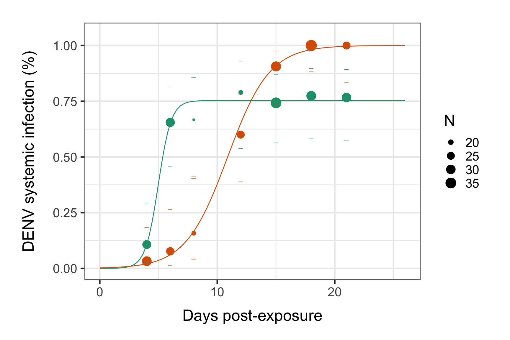
#Save in pdf:
#ggsave(filename = "Systemic_infection_dynamics.pdf", p,width = 16,height = 10)

#Save in svg:
#svglite("Systemic_infection_dynamics.svg", width = 16,height = 10)
#print(p)
#dev.off()
We will soon see how to compare systemic infection dynamics between conditions and assess the impact of each intra-host systemic infection dynamic for each species. Which species will give the most vertebrate infection cases in the field?
Stay tuned :)
Albin Fontaine
Researcher
My main research interests include vector-borne diseases surveillance, interaction dynamics between mosquito-borne pathogens and their hosts, and quantitative genetics applied to mosquito-viruses interactions.