Making maps in R
We will see here how to make nice maps in R with very few lines of code. I am not an expert in GIS, but people have developed nice packages that are doing the job for you. What is here is just a compilation of the work from others. At the end of this tutorial, you will be able to do these maps (and much better ones) by just copy/pasting my code and change the input data.
Let’s go.
Make your 2D map with the ggmap package with only few lines of code
You will need to install and load these packages:
-leaflet -ggmap -ggrepel -ggsn -rgdal
Create your Bounding Box and visualize with a Leaflet interactive map.
We are first going to delineate our map. A bounding box (usually shortened to bbox) is an area defined by two longitudes and two latitudes that usually follow the standard format of min Longitude, min Latitude, max Longitude, max Latitude.
I am here targeting a region in the French Alpes (i.e. La vallée du Valgaudemar, where I used to go hiking) with a bbox of min Longitude: 5.99276974006526 , min Latitude:44.68960794878319 , max Longitude: 6.430718387032721, max Latitude: 44.909422044424076. GPS coordinates are in Decimal Degrees. If your coordinates are in DMS format (Degrees Minutes Seconds), you can easily convert them via dedicated websites, such as: https://www.latlong.net/lat-long-dms.html (this one display the location on a map). You can use the leaflet package to visualize the bbox, I find it very convenient.
# Define bounding box with longitude/latitude coordinates
bbox <- list(
  p1 = list(long = 5.99276974006526, lat = 44.68960794878319),
  p2 = list(long = 6.430718387032721, lat = 44.909422044424076)
)


leaflet() %>%
  addTiles() %>%
  addRectangles(
    lng1 = bbox$p1$long, lat1 = bbox$p1$lat,
    lng2 = bbox$p2$long, lat2 = bbox$p2$lat,
    fillColor = "transparent" ) %>%
  fitBounds(
    lng1 = bbox$p1$long, lat1 = bbox$p1$lat,
    lng2 = bbox$p2$long, lat2 = bbox$p2$lat  )
Is the bounding box ok? Change the GPS coordinate if needed.
Create data to place on the map
We now are going to load the data points we want to place on the map. If you have few locations to map, you can create a data.frame from scratch as below, otherwise you can import a data.frame from a spreadsheet (refer to my tuto: https://www.albinfontaine.com/post/take-your-first-steps-in-r/ )
I here create a data.frame with 4 columns: Locality, Latitude, Longitude and location type.
dat <- data.frame(Locality=c("La Chapelle en Valgaudemar", "Refuge du Gioberney (1 650 m)", "Refuge du Pigeonnier (2 427 m)", "Refuge de Vallonpierre (2 271 m)", "Refuge de L'Olan (2 332 m)", "Lac de Petarel (2 090 m)", "Lac du Lauzon (2 008 m)", "L Olan (3 564 m)"), Latitude=c(44.8166818,44.8409061, 44.8548252, 44.798447, 44.8414665, 44.80153, 44.8450528, 44.859173), Longitude=c(6.1952042,6.2812231,6.2849197, 6.2891739, 6.2043872, 6.16863, 6.2732206, 6.1967294), Type=c("Village", "Shelter", "Shelter", "Shelter", "Shelter", "Lac", "Lac", "Peak"))

dat
## Locality Latitude Longitude Type
## 1 La Chapelle en Valgaudemar 44.81668 6.195204 Village
## 2 Refuge du Gioberney (1 650 m) 44.84091 6.281223 Shelter
## 3 Refuge du Pigeonnier (2 427 m) 44.85483 6.284920 Shelter
## 4 Refuge de Vallonpierre (2 271 m) 44.79845 6.289174 Shelter
## 5 Refuge de L'Olan (2 332 m) 44.84147 6.204387 Shelter
## 6 Lac de Petarel (2 090 m) 44.80153 6.168630 Lac
## 7 Lac du Lauzon (2 008 m) 44.84505 6.273221 Lac
## 8 L Olan (3 564 m) 44.85917 6.196729 PeakPlace markers on the leaflet map.
Colored circles are replacing the location markers. Each color correspond to a location “Type” as referred to the “dat” dataframe. The name of the locality will appear when you clic on it. The type will appear when you place your mouse over the location. We also add a mini.map on the bottom right.
# first attribute a color to each categorical variable

dat$Type <- factor(dat$Type)
Col <- colorFactor(palette = 'Dark2', dat$Type)

leaflet() %>%
  addTiles() %>%
  addRectangles(
    lng1 = bbox$p1$long, lat1 = bbox$p1$lat,
    lng2 = bbox$p2$long, lat2 = bbox$p2$lat,
    fillColor = "transparent" ) %>%
  fitBounds(
    lng1 = bbox$p1$long, lat1 = bbox$p1$lat,
    lng2 = bbox$p2$long, lat2 = bbox$p2$lat  )%>%
addCircleMarkers(data = dat, ~Longitude, ~Latitude, popup = ~as.character(Locality), label = ~as.character(Type), color = ~Col(Type), stroke = FALSE, radius = ~ifelse(Type == "Village", 12, 8), fillOpacity = 0.9) %>%
addMiniMap(tiles = providers$Esri.OceanBasemap, width = 120, height=80)
Now we add a layer control to the top right corner.
# first attribute a color to each categorical variable

groups = as.character(unique(dat$Type))

map = leaflet() %>%
  addTiles() %>%
  addRectangles(
    lng1 = bbox$p1$long, lat1 = bbox$p1$lat,
    lng2 = bbox$p2$long, lat2 = bbox$p2$lat,
    fillColor = "transparent" ) %>%
  fitBounds(
    lng1 = bbox$p1$long, lat1 = bbox$p1$lat,
    lng2 = bbox$p2$long, lat2 = bbox$p2$lat  )

for(g in groups){
  d = dat[dat$Type == g, ]
  map = map %>% addCircleMarkers(data = d, ~Longitude, ~Latitude, popup = ~as.character(Locality), label = ~as.character(Type), color = ~Col(Type), stroke = FALSE, radius = ~ifelse(Type == "Village", 12, 8), fillOpacity = 0.9, group = g)

}

map %>% addLayersControl(overlayGroups = groups, options = layersControlOptions(collapsed = FALSE))
We are now going to add a .gpx hiking track on the map.
track <- plotKML::readGPX("Le-lac-du-Lauzon.gpx")

require(rgdal)
## Le chargement a nécessité le package : rgdal## rgdal: version: 1.5-23, (SVN revision 1121)
## Geospatial Data Abstraction Library extensions to R successfully loaded
## Loaded GDAL runtime: GDAL 3.2.1, released 2020/12/29
## Path to GDAL shared files: /Library/Frameworks/R.framework/Versions/4.0/Resources/library/rgdal/gdal
## GDAL binary built with GEOS: TRUE
## Loaded PROJ runtime: Rel. 7.2.1, January 1st, 2021, [PJ_VERSION: 721]
## Path to PROJ shared files: /Library/Frameworks/R.framework/Versions/4.0/Resources/library/rgdal/proj
## PROJ CDN enabled: FALSE
## Linking to sp version:1.4-5
## To mute warnings of possible GDAL/OSR exportToProj4() degradation,
## use options("rgdal_show_exportToProj4_warnings"="none") before loading rgdal.
## Overwritten PROJ_LIB was /Library/Frameworks/R.framework/Versions/4.0/Resources/library/rgdal/projtrack <- readOGR("randonnee-lac-du-lauzon-valgaudemar.gpx", layer = "tracks", verbose = FALSE)
map %>% addPolylines(data=track) Once in Rstudio, you can export the map as a standalone .html file. Very easy to do, very nice rendering.
Make the 2D map with ggmap.
We first have to load the map via the get_map (ggmap package) function. You can load different type of map. You can refer to the “Cheat sheet” to have a glimpse on the options: https://colauttilab.github.io/EcologyTutorials/ggmapCheatsheet.pdf.
I am using here data from OpenStreetMap (OSM), the collaborative project that create a free editable map of the world. The map will be in the vectorial style (ie. drawing) but the function load a .png. You can load different types of maps, including satellite images, but they are often not free.
Map <- get_map(location=c(left = bbox$p1$long , bottom = bbox$p1$lat, right = bbox$p2$long , top = bbox$p2$lat),source="osm")Here, I assign a color to each type of point.
myColors <- c("black","darkorange","darkgreen","darkblue")
names(myColors) <- levels(factor(dat$Type, levels=c("Village", "Shelter", "Peak", "Lac" )))
colScale <- scale_color_manual(name = "Type",values = myColors)
I am using the “ggsn” package to plot the North arrow and the scalebar.
map <- ggmap(Map)
map <- map + coord_fixed() + theme_minimal(base_size = 20)
## Coordinate system already present. Adding new coordinate system, which will replace the existing one.map <- map + ggtitle("Study area") + colScale
map <- map + geom_point(data=dat, aes(x=Longitude, y=Latitude, color=Type),size=5, alpha=0.9)
map <- map + xlab("Longitude")+ ylab("Latitude")
map <- map + north(location = "topleft", x.min = bbox$p1$long, x.max = bbox$p2$long, y.min = bbox$p1$lat, y.max = (bbox$p2$lat-0.01))
map <- map + ggsn::scalebar(x.min = bbox$p1$long, x.max = bbox$p2$long-0.02, y.min = (bbox$p1$lat+0.01), y.max = bbox$p2$lat, location = "bottomright",transform = TRUE, dist = 2,dist_unit="km", model = "WGS84")
map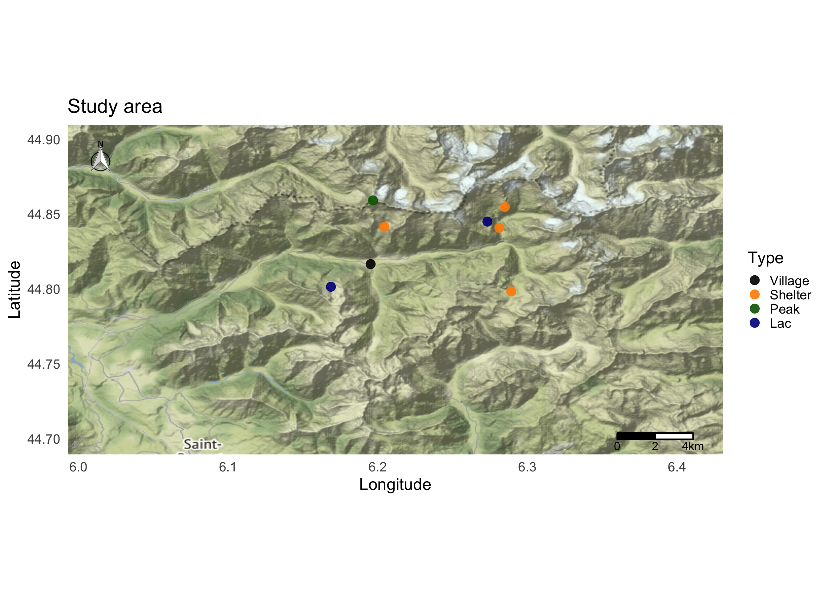
We can add locations using the geom_label_repel function. This function try to avoid label overlapping.
map <- ggmap(Map)
map <- map + coord_fixed() + theme_minimal(base_size = 20)
## Coordinate system already present. Adding new coordinate system, which will replace the existing one.map <- map + ggtitle("Study area") + colScale
map <- map + geom_point(data=dat, aes(x=Longitude, y=Latitude, color=Type),size=5, alpha=0.9)
map <- map + geom_label_repel(size=4, data=dat, aes(x=Longitude, y=Latitude, label = Locality),force = 50, label.size = 0.5)
map <- map + xlab("Longitude")+ ylab("Latitude")
map <- map + north(location = "topleft", x.min = bbox$p1$long, x.max = bbox$p2$long, y.min = bbox$p1$lat, y.max = (bbox$p2$lat-0.01))
map <- map + ggsn::scalebar(x.min = bbox$p1$long, x.max = bbox$p2$long-0.02, y.min = (bbox$p1$lat+0.01), y.max = bbox$p2$lat, location = "bottomright",transform = TRUE, dist = 2,dist_unit="km", model = "WGS84")
map
You can change a lot of options by accessing the functions help (eg. ?north) to the graph that suit you. You can notice that I added some values to the x.min/max and y.min/max to place the scalebar. You will probably to ajust that manually, but it shouldn’t be a big deal.
Save the map
require(svglite)
svglite("Map.svg", width = 10,height = 10)
print(map)
dev.off()
Make your 3D map easily with the Geoviz and rayshader package
You will need to load and install these packages:
-rayshader -rayrender -geoviz -raster
You can make astonishing 3D maps with very few line of codes with the Rayshader package developped by Tyler Morgan (https://github.com/tylermorganwall/rayshader/blob/master/README.md). I will not extend to much on the abilities of this package here because others have made very nice tutos about it. For exemple you can refer to https://wcmbishop.github.io/rayshader-demo/ or https://www.davidsolito.com/post/a-rayshader-base-tutortial-bonus-hawaii/.
The first thing that you will need is elevation data. They usually come in a form of a raster (pixel) image.
Option 1:
One option to collect such data is this website: https://portal.opentopography.org/datasets
Once on the website data map, zoom on your region of interest (it can be outside of the colored points, color points only refers to areas with high-quality topographic data available, but other region are fine). Clic “Select a region” to your left hand side and make your boundary box.
Clic raster and select GeoTIFF format with maximum resolution.
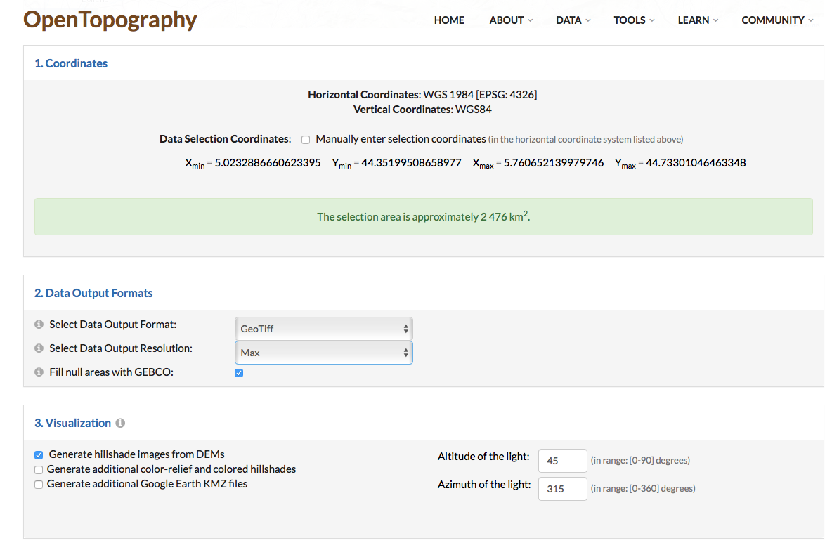
Download the file, mine appears as “output_gmrt.tif”
We load this file with the raster function and set up a coordinate reference system. Just copy/paste it is going to be ok :).
elev_img <- raster(x = "output_gmrt.tif")
proj4string(elev_img) <- CRS('+proj=longlat +datum=WGS84 +no_defs')
Option 2:
An alternative would be to use the Geoviz package that allows you to download Digital Elevation Model with the mapzen_dem(lat, long, square_km) function. Very easy, all is done with one line of code: I have to use suppressWarnings() function because Geoviz functions give me a lot of warnings. It doesn’t seem to have any effect, it is just warnings. *Unfortunatly, this solution does not work anymore since I updated the rayshader package.
Now that we get our digital elevation data (ie. elev_img), we need an overlay image. You can find one by your own (eg. a nice satellite image), or just use the slippy_overlay function (from the geoviz package) that will do the job for you.
suppressWarnings(overlay <- slippy_overlay(elev_img, image_source = "stamen", image_type = "terrain-background", png_opacity = 1))We now do the Rayshader magic:
Convert raster image to matrix:
#And convert it to a matrix:
elev_matrix = raster_to_matrix(elev_img)
calculate rayshader layers and plot the map:
ambmat <- ambient_shade(elev_matrix)
raymat <- ray_shade(elev_matrix)
watermap <- detect_water(elev_matrix)


#We use another one of rayshader's built-in textures:
elev_matrix %>%
  sphere_shade(texture = "desert") %>%
  add_water(watermap, color = "desert") %>%
  add_shadow(raymat, 0.5) %>%
  add_shadow(ambmat, 0) %>%
  plot_map()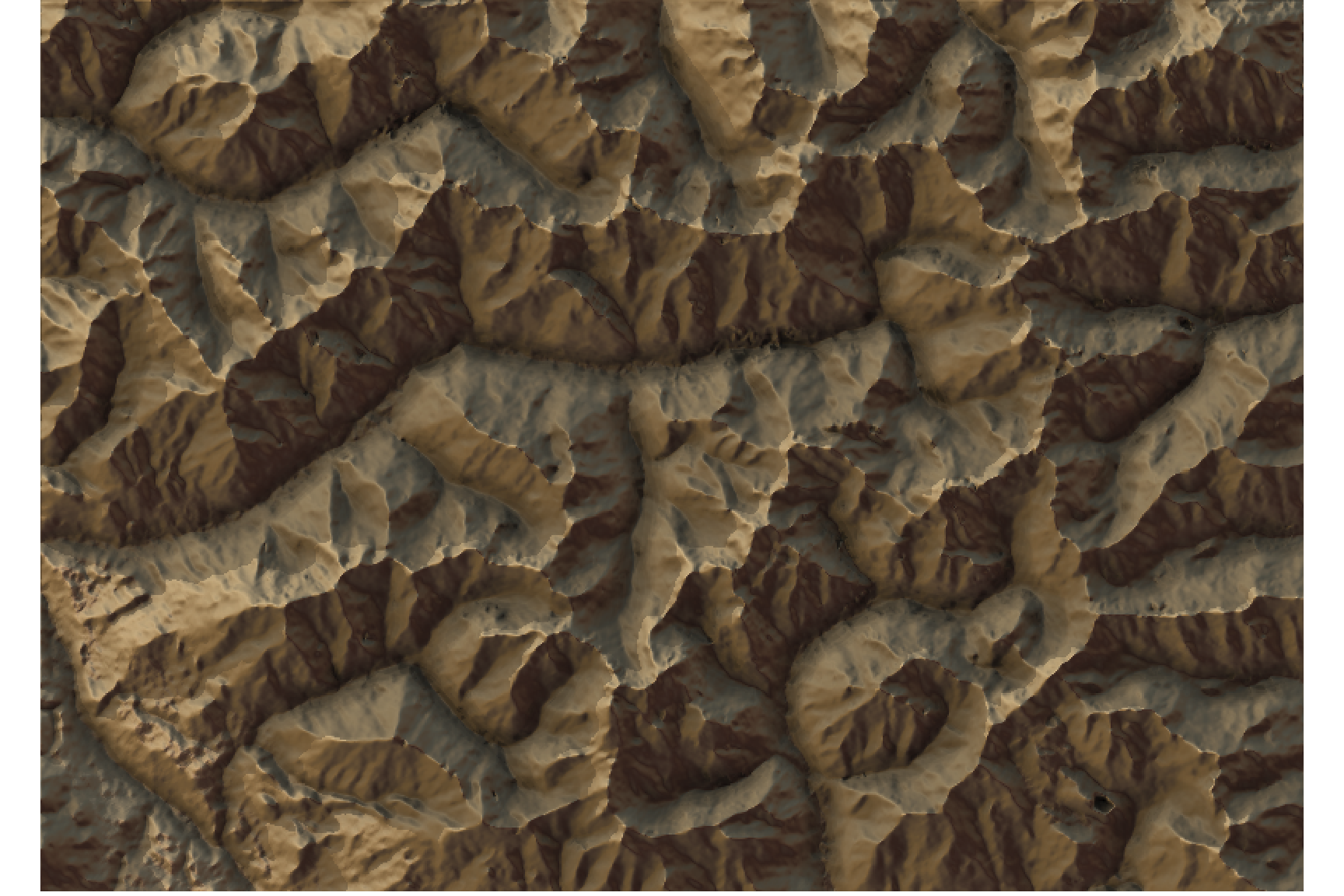
We can add the image overlay. The alphalayer option sets the transparency value (between 0 and 1, the lower is the more transparent).
elev_matrix %>%
  sphere_shade(texture = "desert") %>%
  add_water(watermap, color = "desert") %>%
  add_shadow(raymat, 0.5) %>%
  add_shadow(ambmat, 0) %>%
  add_overlay(overlay, alphalayer = 0.7) %>%
  plot_map()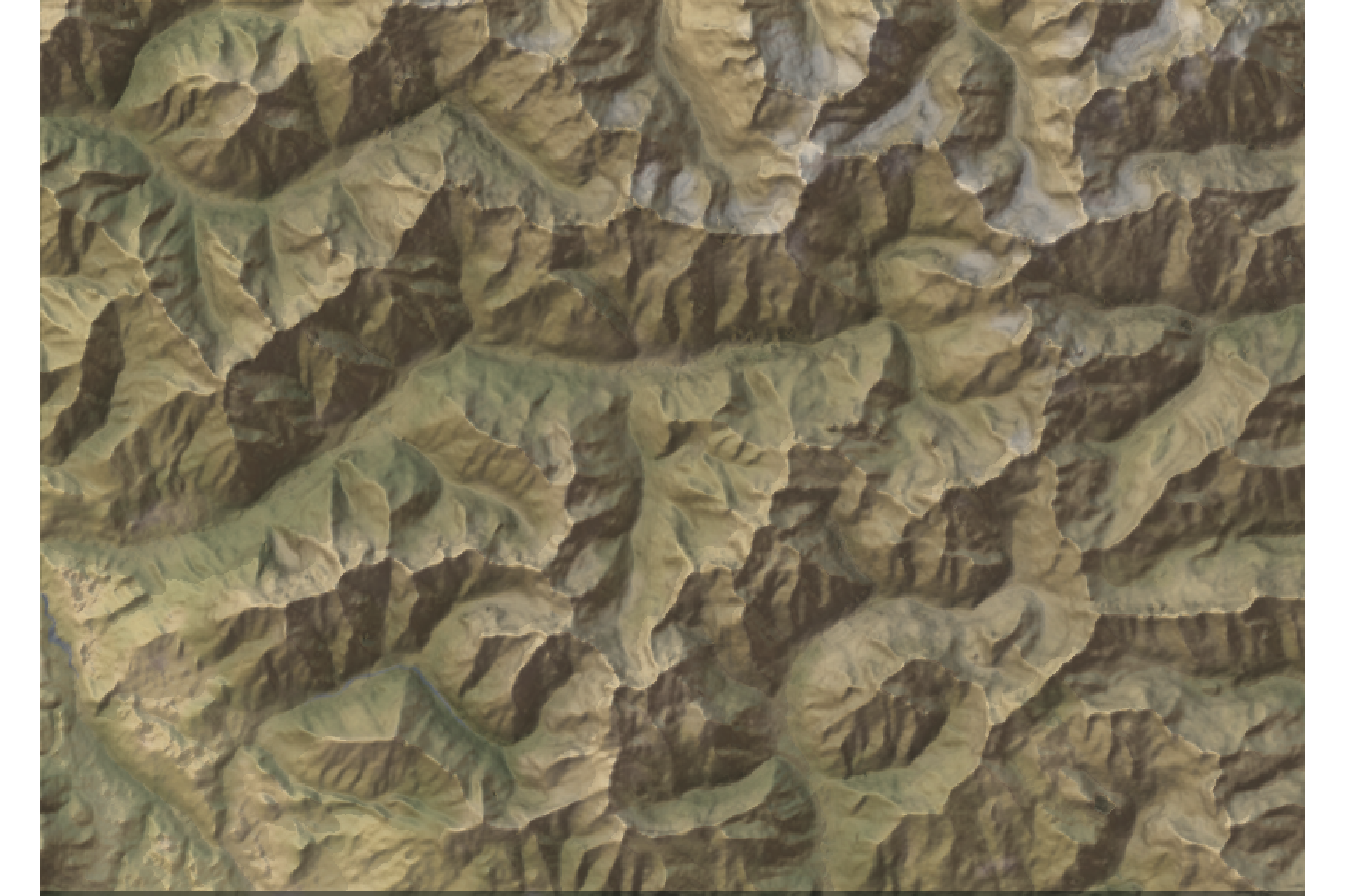
Make the 3D plot and add labels with the render_label function.
zscale <- raster_zscale(elev_img)
rgl::clear3d()

elev_matrix %>%
  sphere_shade(texture = "desert") %>%
  add_water(watermap, color = "imhof4") %>%
  add_shadow(raymat, 0.5) %>%
  add_shadow(ambmat, 0.5) %>%
  add_overlay(overlay, alphalayer = 0.8) %>%
  plot_3d(elev_matrix, zscale = zscale, windowsize = c(900, 900),
          water = F,  theta = 0, phi = 20, zoom = 0.8, fov = 40)

render_label(elev_matrix, lat =44.81668, long = 6.195204, altitude = 7000, extent=attr(elev_img, "extent"), freetype=T, zscale = zscale, text = "La Chapelle en Valgaudemar", dashed = F, textsize = 1, linewidth = 2, textcolor = "black", linecolor="black")

render_snapshot(clear = TRUE)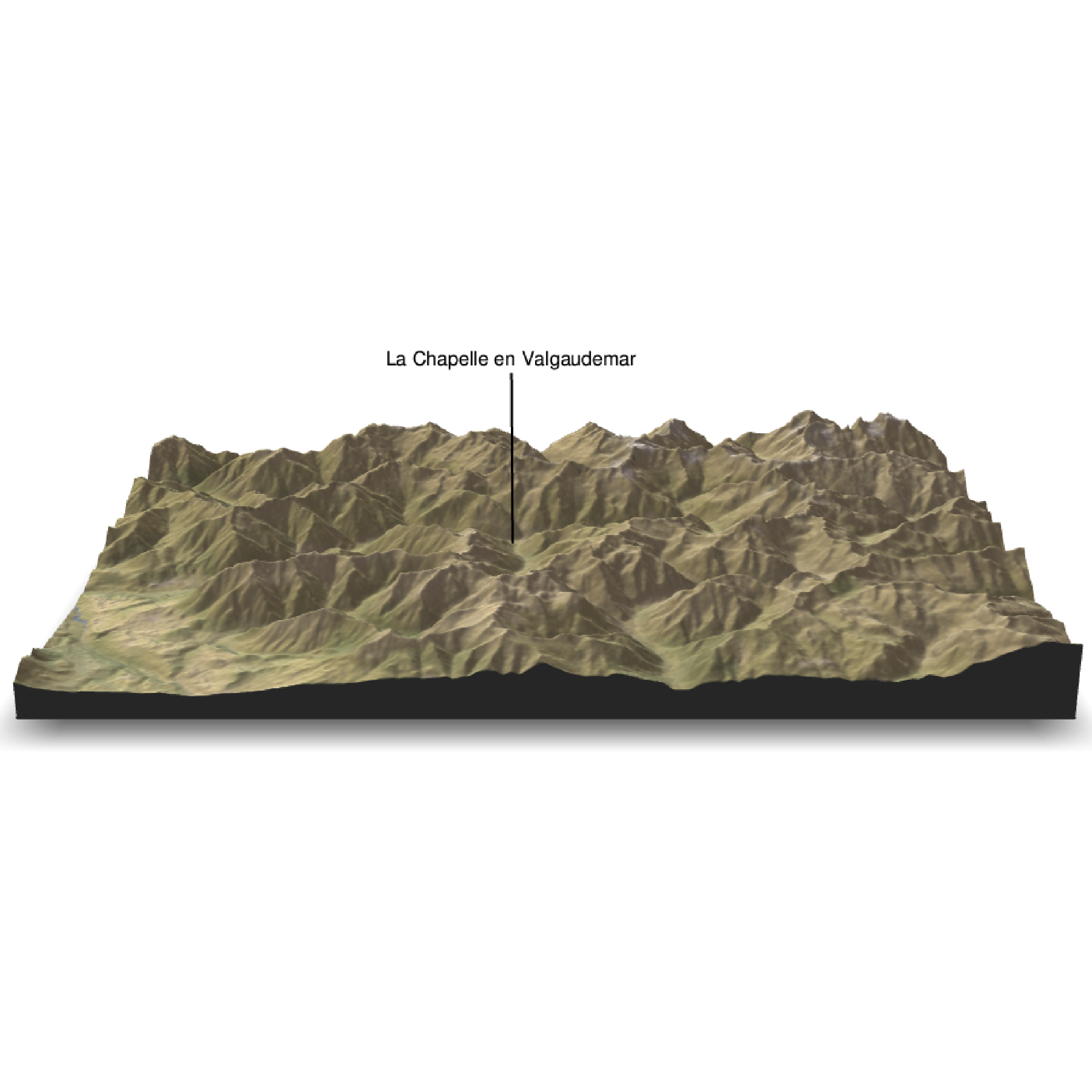
We can add a scalebar
zscale <- raster_zscale(elev_img)
rgl::clear3d()

elev_matrix %>%
  sphere_shade(texture = "desert") %>%
  add_water(watermap, color = "imhof4") %>%
  add_shadow(raymat, 0.5) %>%
  add_shadow(ambmat, 0.5) %>%
  add_overlay(overlay, alphalayer = 0.8) %>%
  plot_3d(elev_matrix, zscale = zscale, windowsize = c(800, 800),
          water = F,  theta = 0, phi = 20, zoom = 0.8, fov = 40)

render_label(elev_matrix, lat =44.81668, long = 6.195204, altitude = 7000, extent=attr(elev_img, "extent"), freetype=T, zscale = zscale, text = "La Chapelle en Valgaudemar", dashed = F, textsize = 1, linewidth = 2, textcolor = "black", linecolor="black")

render_scalebar(limits=c(0, 5, 10),label_unit = "km",position = "W", y=50,  scale_length = c(0.33,1))

render_snapshot(clear = TRUE)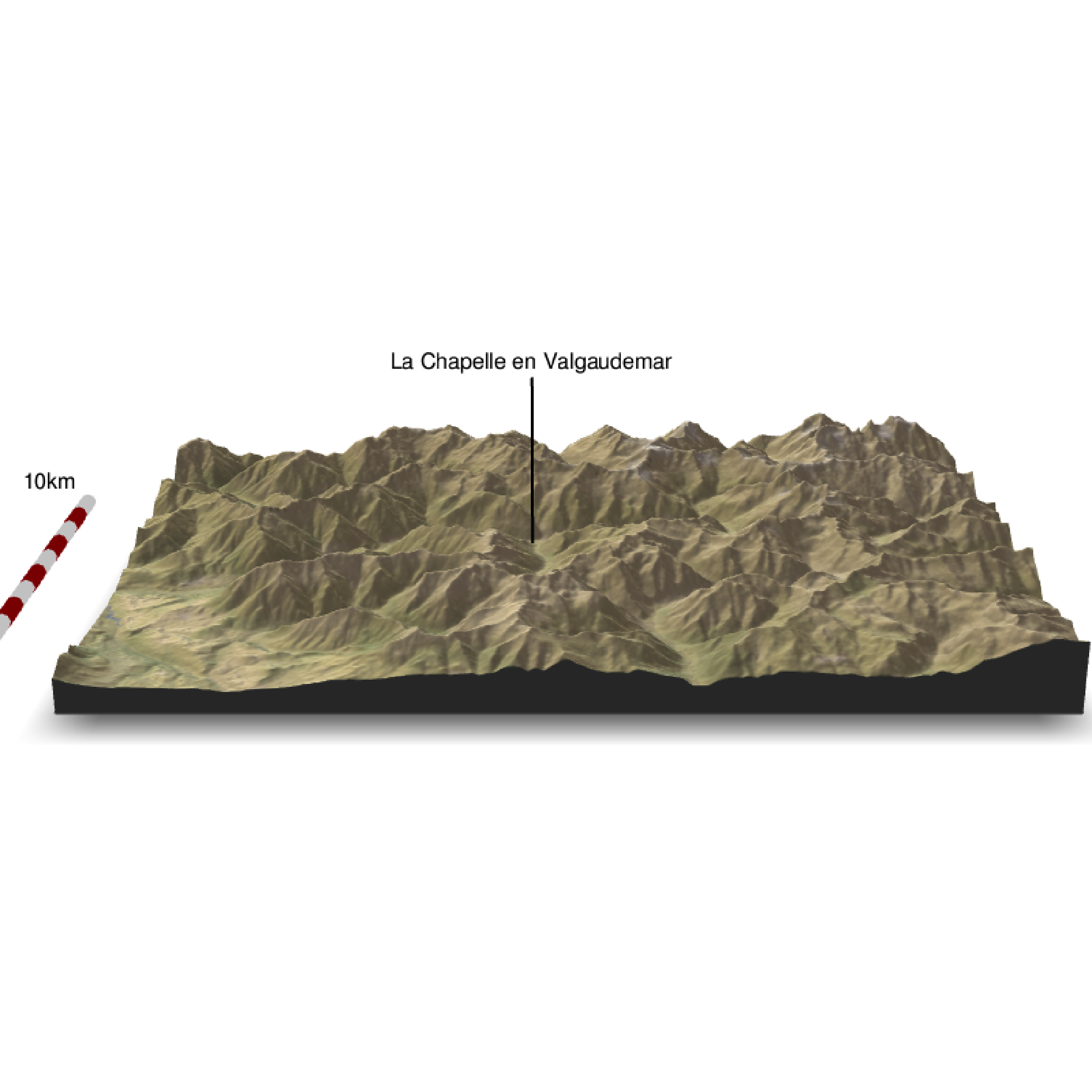
You can play with the theta, phi, zoom and fov options to place the point of view…and the other many options (type ?plot_3d() to access all the options) or you can have a look in the Rayshader webpage: https://www.rayshader.com
zscale <- raster_zscale(elev_img)
rgl::clear3d()

elev_matrix %>%
  sphere_shade(texture = "desert") %>%
  add_water(watermap, color = "imhof4") %>%
  add_shadow(raymat, 0.5) %>%
  add_shadow(ambmat, 0.5) %>%
  add_overlay(overlay, alphalayer = 0.8) %>%
  plot_3d(elev_matrix, zscale = zscale, windowsize = c(800, 800),
          water = F,  theta = 60, phi = 30, zoom = 0.6, fov = 0)

render_label(elev_matrix, lat =44.81668, long = 6.195204, altitude = 9000, extent=attr(elev_img, "extent"), freetype=T, zscale = zscale, text = "La Chapelle en Valgaudemar", dashed = F,  linewidth = 2, textcolor = "black", linecolor="black")

render_label(elev_matrix, lat =44.84091, long = 6.281223, altitude = 4000, extent=attr(elev_img, "extent"), freetype=T, zscale = zscale, text = "Refuge du Gioberney (1 650 m)", dashed = F, linewidth = 2, textcolor = "black", linecolor="Darkorange")

render_label(elev_matrix, lat =44.84147, long = 6.204387, altitude = 9000, extent=attr(elev_img, "extent"), freetype=T, zscale = zscale, text = "Refuge de L'Olan (2 332 m)", dashed = F, linewidth = 2, textcolor = "black", linecolor="Darkorange")

render_label(elev_matrix, lat =44.85483, long = 6.284920, altitude = 9000, extent=attr(elev_img, "extent"), freetype=T, zscale = zscale, text = "Refuge du Pigeonnier (2 427 m)", dashed = F, linewidth = 2, textcolor = "black", linecolor="Darkorange")

render_label(elev_matrix, lat =44.79845, long = 6.289174, altitude = 2000, extent=attr(elev_img, "extent"), freetype=T, zscale = zscale, text = "Refuge de Vallonpierre (2 271 m)", dashed = F, linewidth = 2, textcolor = "black", linecolor="Darkorange")

render_snapshot(clear = TRUE)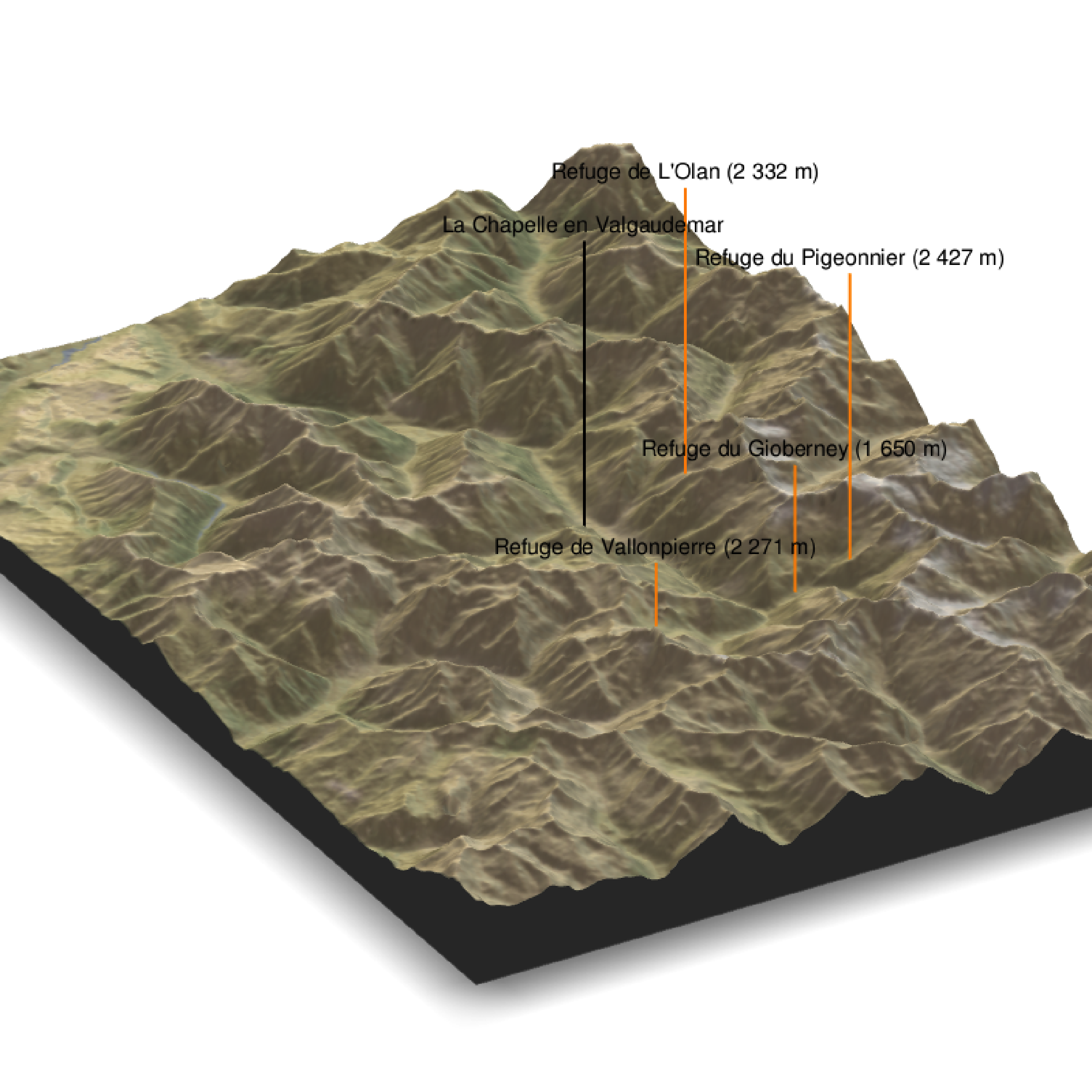
With a circle baseshape:
zscale <- raster_zscale(elev_img)
rgl::clear3d()

elev_matrix %>%
  sphere_shade(texture = "desert") %>%
  add_water(watermap, color = "imhof4") %>%
  add_shadow(raymat, 0.5) %>%
  add_shadow(ambmat, 0.5) %>%
  add_overlay(overlay, alphalayer = 0.8) %>%
  plot_3d(elev_matrix, zscale = zscale, windowsize = c(800, 800),
          water = F,  theta = 60, phi = 30, zoom = 0.6, fov = 0, baseshape="circle")

render_label(elev_matrix, lat =44.81668, long = 6.195204, altitude = 9000, extent=attr(elev_img, "extent"), freetype=T, zscale = zscale, text = "La Chapelle en Valgaudemar", dashed = F,  linewidth = 2, textcolor = "black", linecolor="black")

render_label(elev_matrix, lat =44.84091, long = 6.281223, altitude = 4000, extent=attr(elev_img, "extent"), freetype=T, zscale = zscale, text = "Refuge du Gioberney (1 650 m)", dashed = F, linewidth = 2, textcolor = "black", linecolor="Darkorange")

render_snapshot(clear = TRUE)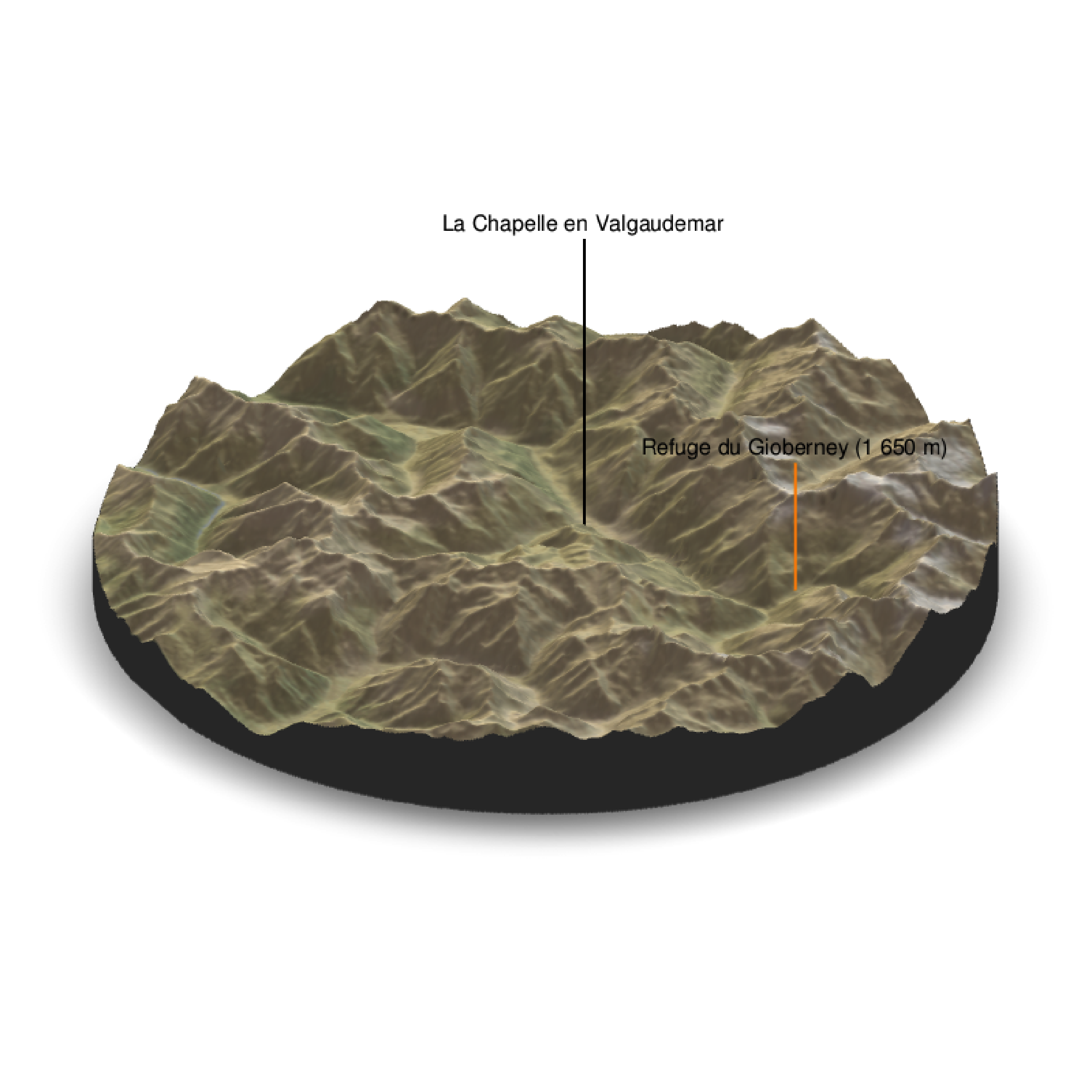
Once your are done, you can save your image with render_snapshot(“image_name”, clear=TRUE), it will save a .png image in your work directory.
We can also plot tracks (hiking, mountain biking, etc…)
track <- plotKML::readGPX("randonnee-lac-du-lauzon-valgaudemar.gpx")

latitude <- as.data.frame(track$tracks[[1]])$lac.lauzon.lat
longitude <- as.data.frame(track$tracks[[1]])$lac.lauzon.lon
altitude <- as.numeric(as.data.frame(track$tracks[[1]])$lac.lauzon.ele)

zscale <- raster_zscale(elev_img)
rgl::clear3d()

elev_matrix %>%
  sphere_shade(texture = "desert") %>%
  add_water(watermap, color = "imhof4") %>%
  add_shadow(raymat, 0.5) %>%
  add_shadow(ambmat, 0.5) %>%
  add_overlay(overlay, alphalayer = 0.8) %>%
  plot_3d(elev_matrix, zscale = zscale, windowsize = c(800, 800),
          water = F,  theta = 30, phi = 30, zoom = 0.2, fov = 100)

render_path( extent=attr(elev_img, "extent"), lat=latitude, long=longitude, altitude=altitude, zscale=zscale-1.2, color="red", antialias=TRUE, linewidth = 5 )

render_label(elev_matrix, lat =44.81668, long = 6.195204, altitude = 4000, extent=attr(elev_img, "extent"), freetype=T, zscale = zscale, text = "La Chapelle en Valgaudemar", dashed = F,  linewidth = 2, textcolor = "black", linecolor="black")

render_label(elev_matrix, lat =44.84091, long = 6.281223, altitude = 3000, extent=attr(elev_img, "extent"), freetype=T, zscale = zscale, text = "Refuge du Gioberney (1 650 m)", dashed = F, linewidth = 2, textcolor = "black", linecolor="Darkorange")

render_snapshot(clear = TRUE)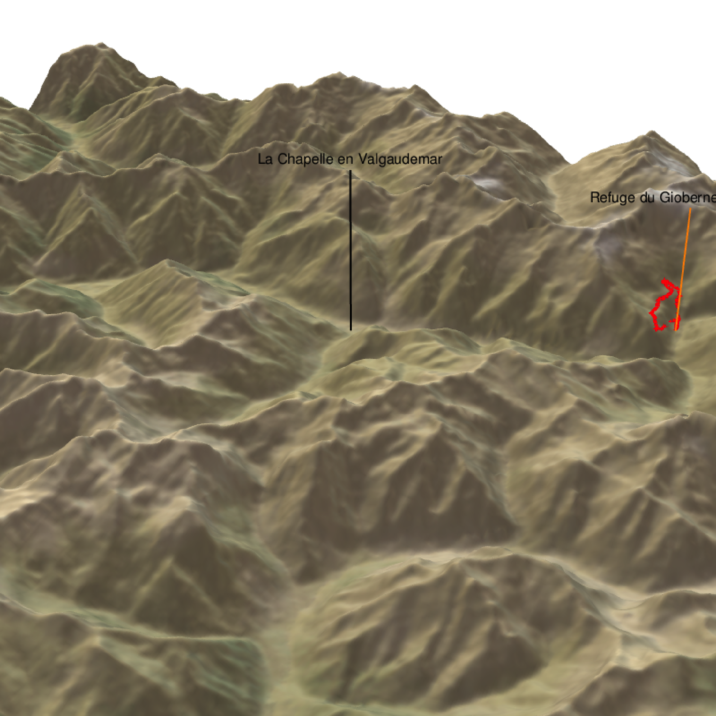
All you have to do is to modify the input data to built your own map !!!
Make your choropleth map
-dplyr -stringr -rgeos -rayshader -viridis
A choropleth map is a map in which areas are shaded or patterned in proportion to a statistical variable. It is more or less a heat map with geographic coordinates. Choropleth maps provide an easy way to visualize a value across a geographic area or to show the level of variability within a region. (https://en.wikipedia.org/wiki/Choropleth_map)
Here, we are going to work with shapefiles. Shapefile is a geospatial vector data format for geographic information system (GIS) softwares. You can download them from dedicated server. It is not always straightforward to find. You can first give a try on this one : https://www.diva-gis.org/gdata
One shapefile comes with 3 mandatory files: .shp — shape format; the feature geometry itself. .shx — shape index format; a positional index of the feature geometry to allow seeking forwards and backwards quickly. .dbf — attribute format; columnar attributes for each shape.
All my files are in the directory “AfricanCountries” at the root of my working directory. I can load them with the shapefile function from the “raster” package.
Here are the few lines of code that you would need to load and display a shapefile.
Africancountries <- shapefile(x = "AfricanCountries/AfricanCountires.shp")

#check if there are invalid geometries & correct that (from https://stackoverflow.com/questions/46003060/error-using-region-argument-when-fortifying-shapefile)

rgeos::gIsValid(Africancountries) #returns FALSE
FALSE [1] FALSEAfricancountries <- rgeos::gBuffer(Africancountries, byid = TRUE, width = 0)
rgeos::gIsValid(Africancountries) #returns TRUEFALSE [1] TRUEI only select “Primary land”:
Africancountries <- subset(Africancountries, Land_Type=="Primary land")

#From https://stackoverflow.com/questions/30790036/error-istruegpclibpermitstatus-is-not-true
library(rgdal)
library(maptools)
if (!require(gpclib)) install.packages("gpclib", type="source")
gpclibPermit()
FALSE [1] TRUE# Convert shapefile to format ggmap can work with
Africancountries_polys = fortify(Africancountries, region = "COUNTRY")
map.test <- ggplot(Africancountries_polys, aes(long,lat,group=group))
map.test <- map.test + geom_polygon(color="darkgrey", fill="white")
map.test <- map.test + coord_fixed() + theme_minimal()
map.test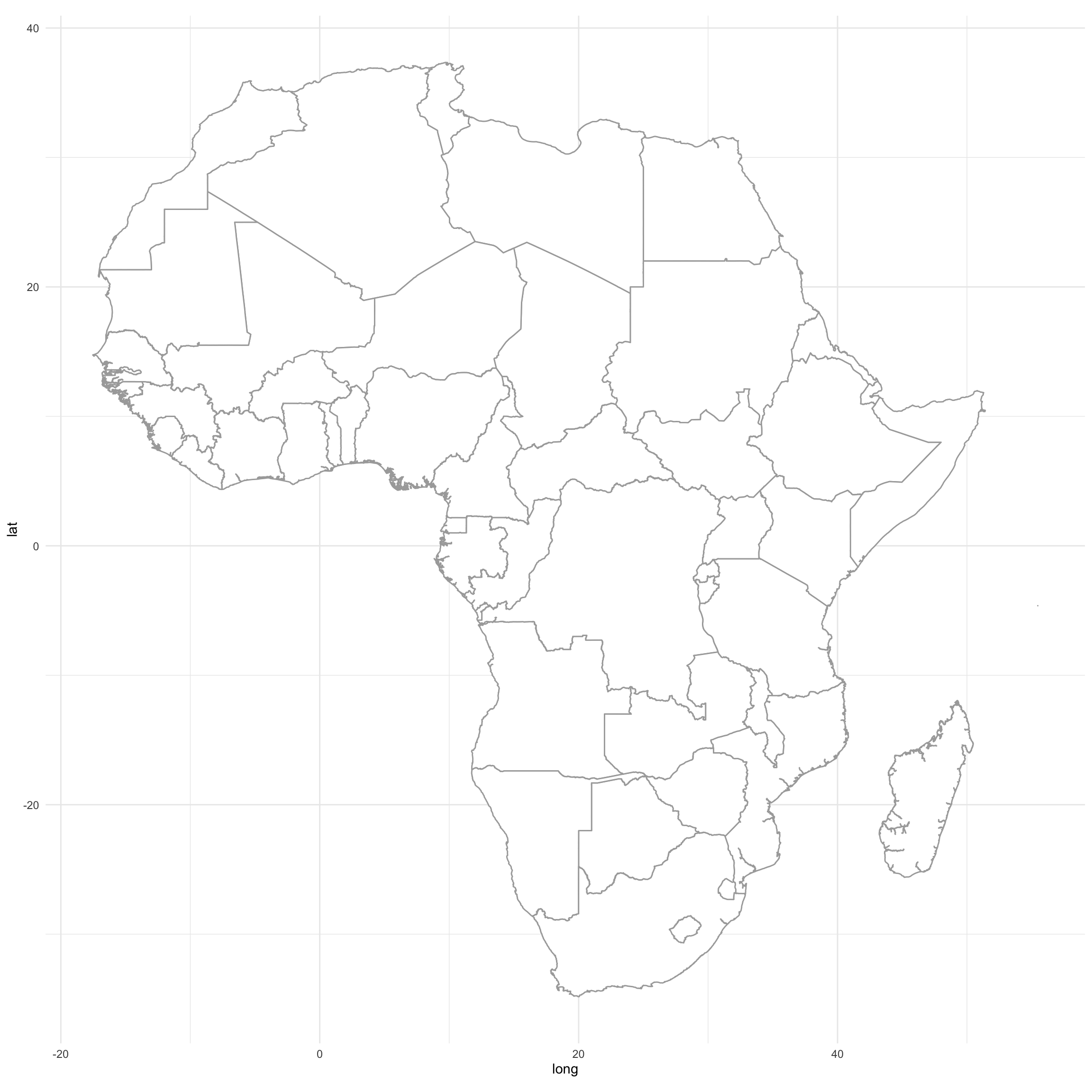
I downloaded population data from the net. It is population data for some African countries. I load them as a data.frame with 3 columns: the Country name, the number of inhbitants and population density expressed as Person per square kilometers. I replaced empty spaces by the "_" symbol to load the data as text (tab delimited) format. I then have to replace back the white spaces so that the countries names match the ones from the shapefile.
Population <- read.table("Population_Africa.txt", h=T )

#I now have to replace "_" by a white space to match country names in the shapefile.
require(stringr)
Population$Countries <- str_replace(Population$Countries, "_", " ")

head(Population)
FALSE Countries Population Density
FALSE 1 Algeria 43851044 18
FALSE 2 Angola 32866272 26
FALSE 3 Benin 12123200 108
FALSE 4 Botswana 2351627 4
FALSE 5 Burkina Faso 20903273 76
FALSE 6 Burundi 11890784 463This is how my data looks like.
#Merge data with the shapefile:
map.df <- left_join(Africancountries_polys, Population, by=c("id"="Countries"))

require(viridis)

map <- ggplot(map.df, aes(long,lat,group=group, fill = Density))
map <- map + geom_polygon(color="white")
map <- map + coord_fixed() + theme_minimal() + scale_fill_viridis()
map <- map
map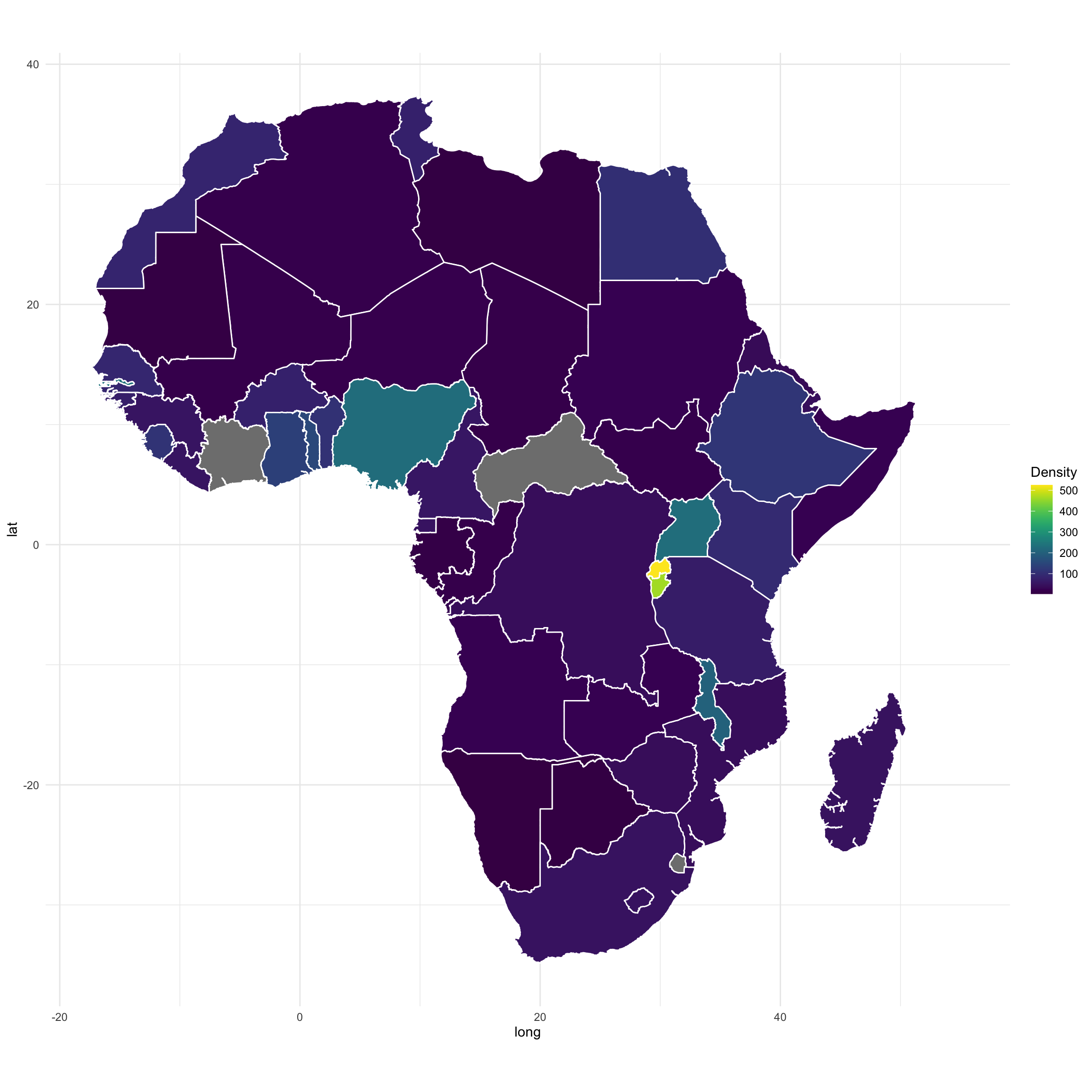
I got an issue (no data) for 2 countries due to special characters or other name mismatch between the shapefile and my data file.
We can also map the population in number of inhabitants. I am using a log10 transformation on the data.
#Merge data with the shapefile:
map.df <- left_join(Africancountries_polys, Population, by=c("id"="Countries"))

require(viridis)

map <- ggplot(map.df, aes(long,lat,group=group, fill = log10(Population)))
map <- map + geom_polygon(color="black")
map <- map + coord_fixed() + scale_fill_viridis()
map <- map
map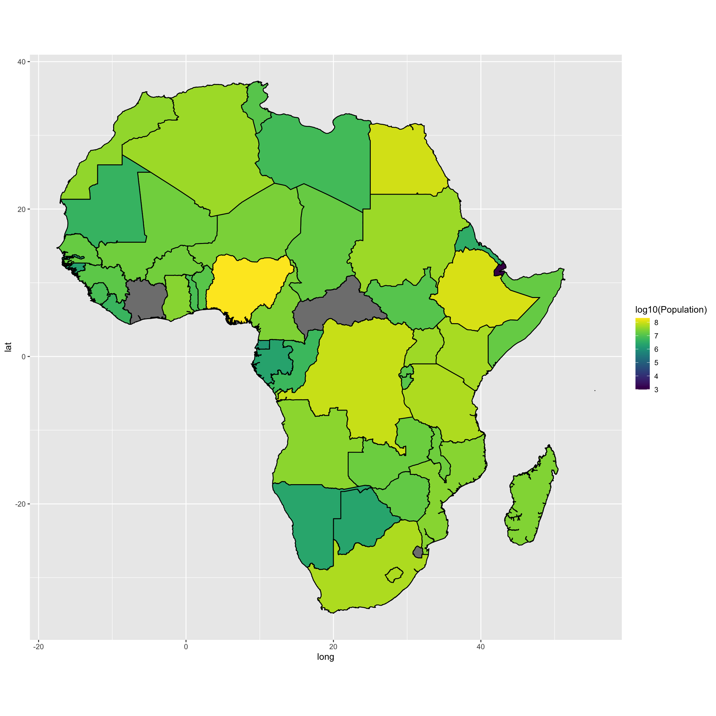
Albin Fontaine
Researcher
My main research interests include vector-borne diseases surveillance, interaction dynamics between mosquito-borne pathogens and their hosts, and quantitative genetics applied to mosquito-viruses interactions.