Take your first steps in R
You are willing to learn how to code in R but you are not familiar with this code? You don’t even know what R or a computing language is and what it can be used for?
This tuto is dedicated to you.
At the end of this short tutorial, you will be able to load your data, manipulate them and make nice ggplot2 charts.
Let’s start!
 Image from https://github.com/allisonhorst/stats-illustrations
What is R and what can you do with it?
R is a computing language and a free software environment for statistical computing and graphics (https://www.r-project.org/about.html). It provides a wide variety of statistical and graphical techniques. The core program comes with open-source (free) packages that can be loaded to have access to a large choice of add-ons developped by other peoples. If you want to do something on a computer, there is probably a package in R for that. You can have a look at this site to have a quick insight of what you can do regarding data visualization: https://www.r-graph-gallery.com.
R and Rstudio installation.
First of all, lets begin by installing R from the The Comprehensive R Archive Network (CRAN). CRAN is a network of ftp and web servers around the world that store identical, up-to-date, versions of code and documentation for R. You can go to the https://cran.r-project.org webpage and follow the instructions.
That is a good first step, but the base R installation is a bit rough to use. We will used RStudio as an integrated development environment (IDE) for R. An IDE is a software that is built specially to help us to write codes efficiently. It has a lot of cool stuffs that can make our life easier. You can download Rstudio and install it from https://rstudio.com/products/rstudio/. RStudio is available in open source and runs on the desktop (Windows, Mac, and Linux). Make sure that you select the desktop version.
Open Rstudio. You should have something like this on your screen:
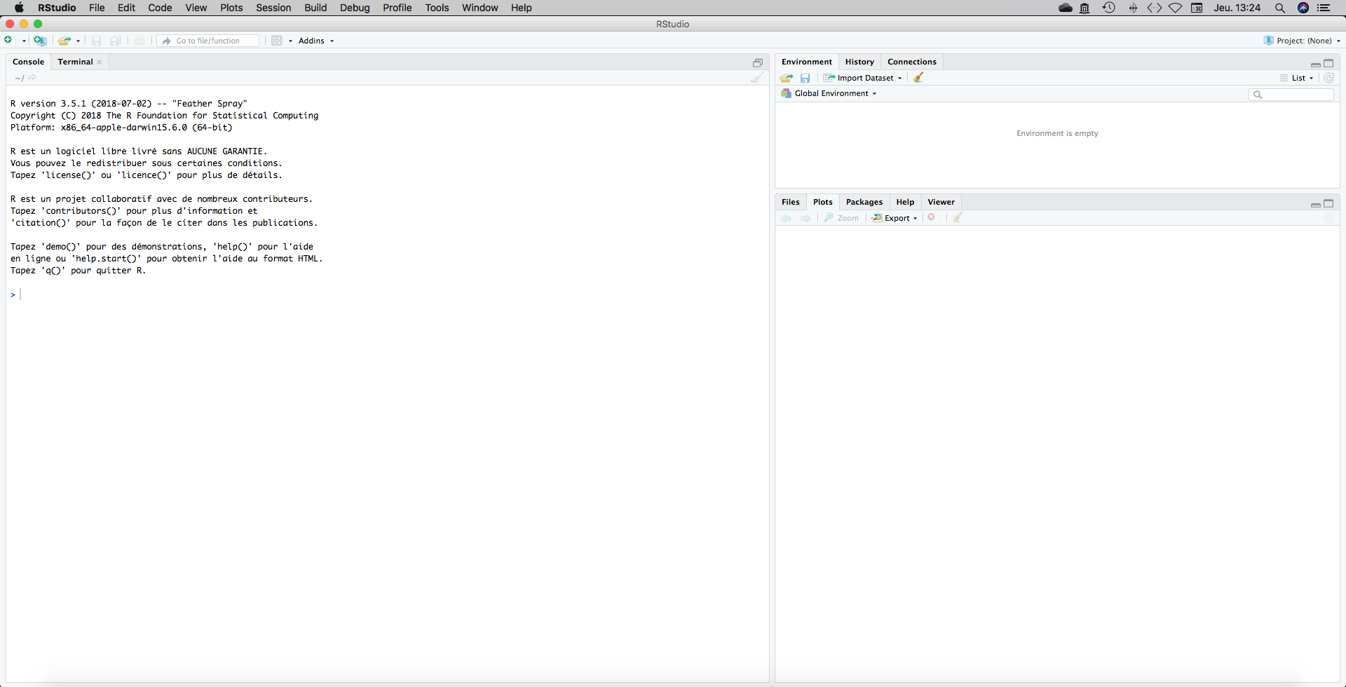
There is three panels.
The top-right panel gives informations about the “Environment”. It is empty for the while.
The bottom-right panel gives informations about “Files”, “Plots”, “Packages”, “Help” and “Viewer”. “Plot” is selected as default and is empty. This is where plots will be displayed. You can have a look a the “Files” tab which give you informations about the folders and directories inside your computer. We will see the other tab later.
The panel called “console” on the left side is the one that will concern us particularly. It has some text which tell you some infos, like the R version that is installed on your computer. You can see the prompt “>” that is waiting for instructions. Let’s focus on this console panel.
R is a calculator
You can type 1 + 2 after the “>” on the console and press enter.
1 + 2## [1] 3The result of our addition (ie 3) should have appeared on the console. That is cool right?
Use of variables
Now we can put “1 + 2” into a variable that we will name “variable”.
Be aware of the “<-” sign which means 1 + 2 is going inside the object named “variable” (this arrow-like shape is pretty self explanatory)
variable <- 1 + 2Nothing happened. Nothing? Not quite! The variable “variable” appeared in your “Environment”" tab. Now type object on the console. The content of the object (ie 3) should appear.
variable## [1] 3Of couse the name variable can be replace by somthing else. You are free to use everything you want, provided it was not used before (not already present in your Environment tab) Otherwise you would overwrite the variable. A variable has to be begin with a letter. You can use plain text (R is case sensitive), or a mix of text and number with “.” or "_" as separator. But NEVER intruce spaces in a variable name.
toto <- 1 + 2
toto
## [1] 3It is time to learn you first trick. You can use the brackets “()” to display on the terminal the content of the object you are creating.
(toto <- 1 + 2)## [1] 3At this stage, you might grab an essential asset of a computing language. It will allow you to implement a serial of tasks on your data based on command lines. These lines, organized in a script, will be used to load, transform, model, and visualize your data.
Create your first script
Go to File, New file, R script.
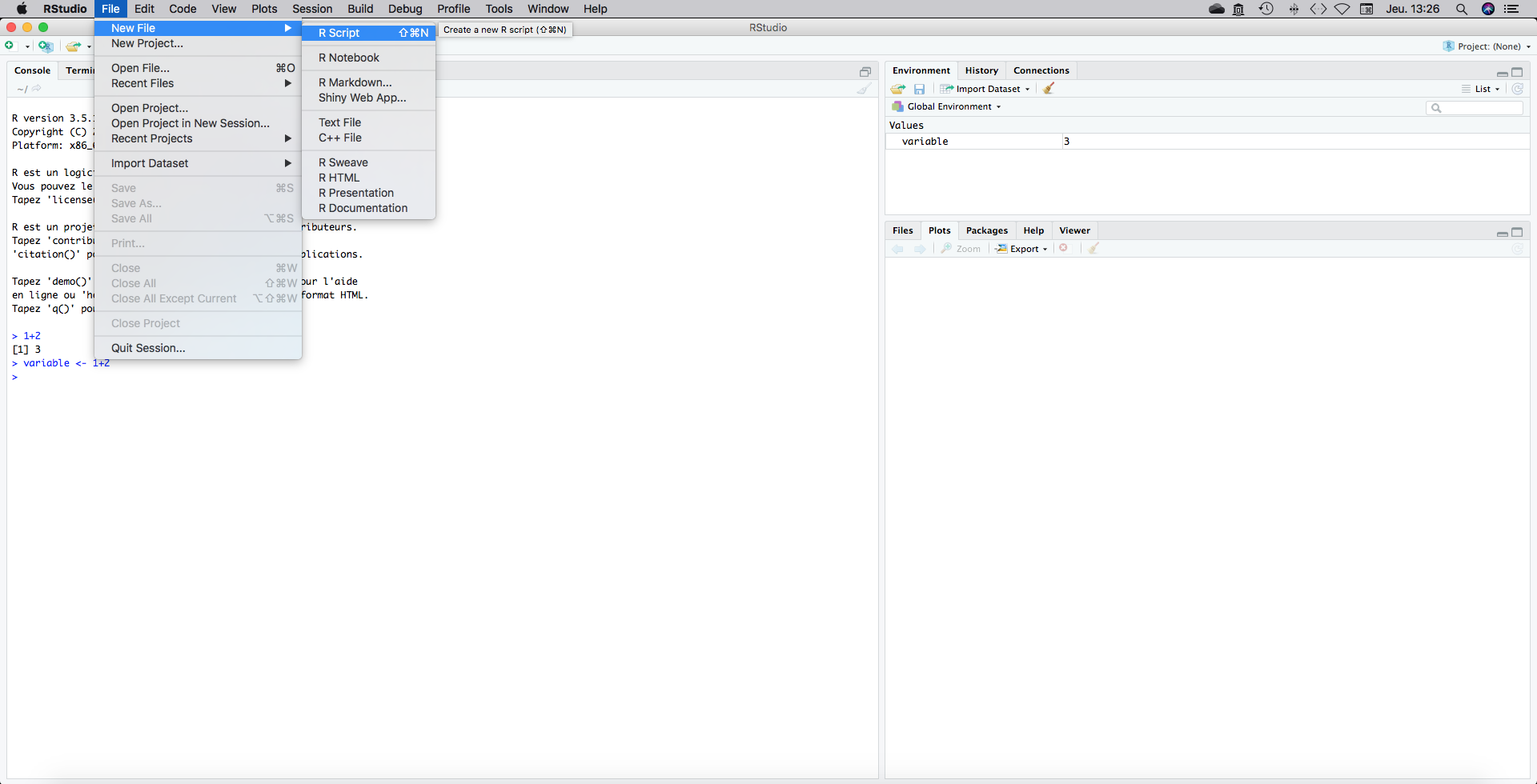
A fourth panel should have appeared on the top-left part of your screen. This is a blank page on which you will write your code. This code can be executed (feeded to the console) line by line, for a batch of consecutive several lines or entirely.
Try it. Type the following code on your script. Then click to place the cursor on your text line and press cmd+enter“(Mac) or”ctrl+enter" (PC). That means that you clic just after (object <- 1 + 2), then put your finger on the “ctrl” key and while your finger is still holding the “ctrl” press the “enter” key. The line code on your script will be run on your console. You can also use the “Run” buttom on the top.
(variable <- 1 + 2)## [1] 3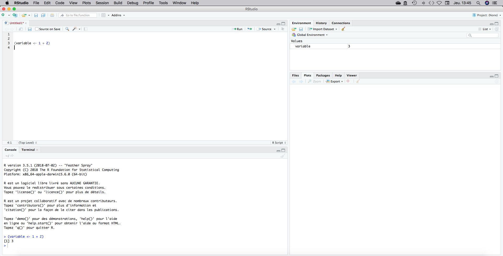
We will start by saving our script to a directory. Go to File, save as…and choose a directory. You can create it from your “Files” panel or by just creating a folder somewhere as you usually do.
Now we need to set our work directory file path. It would tell R where is located your script. To do that click on Session, Set Work Directory, To source File Location. It will tell R to work on the folder where the script is saved.
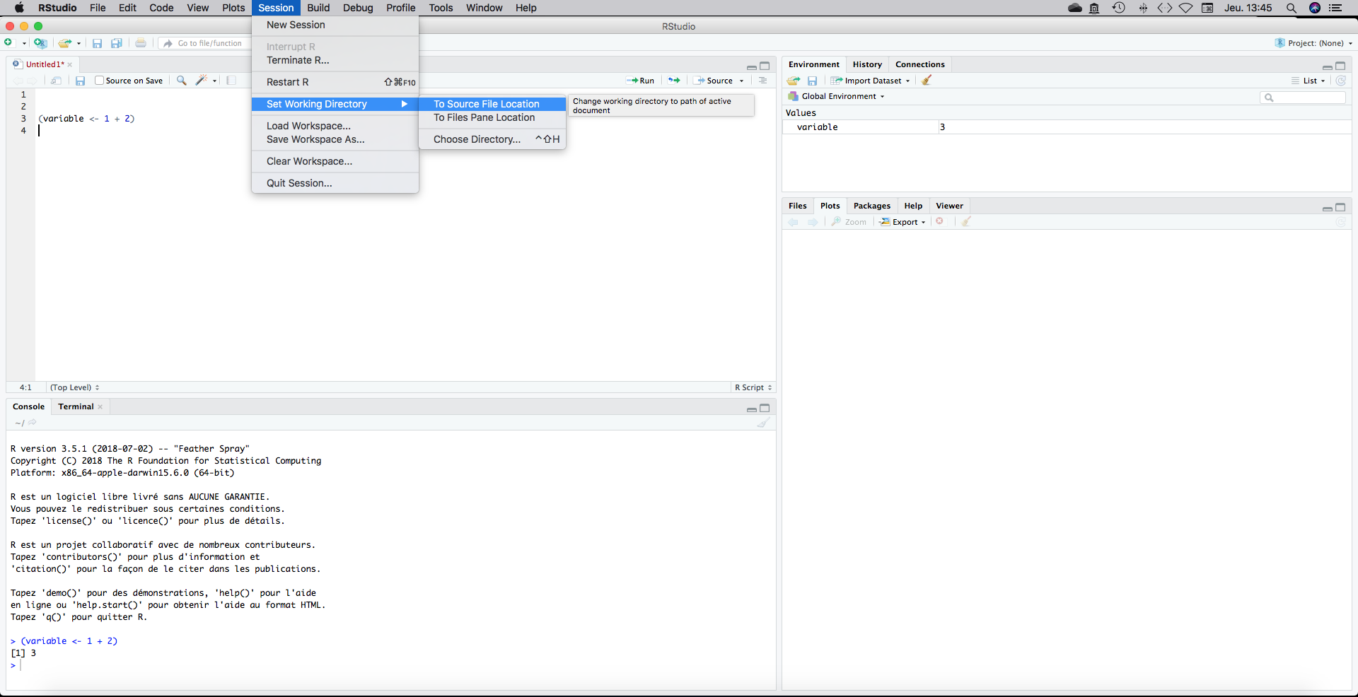
A setwd(“yourpath”) line appears in the console. Copy and paste it on the top of your script. Each time you will open this script, R would know where to find the data if you save them in the same directory than the .R script.
Install and load packages
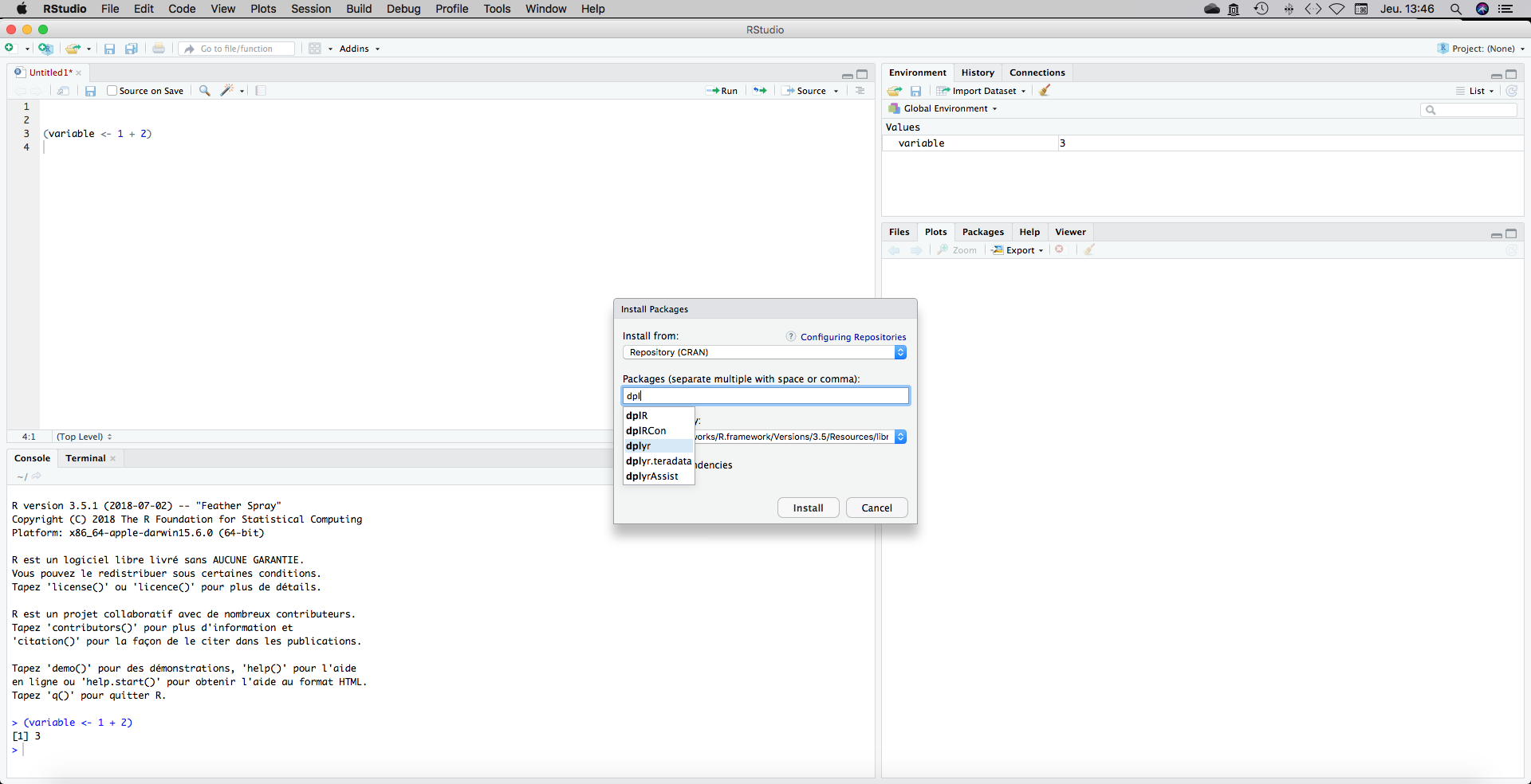
We now have a script with an indication towards our working directory in the first line. What I usually do is loading my packages just after the setwd() on the top of my document. To install a package go to Tools, Install Packages and type the package name.
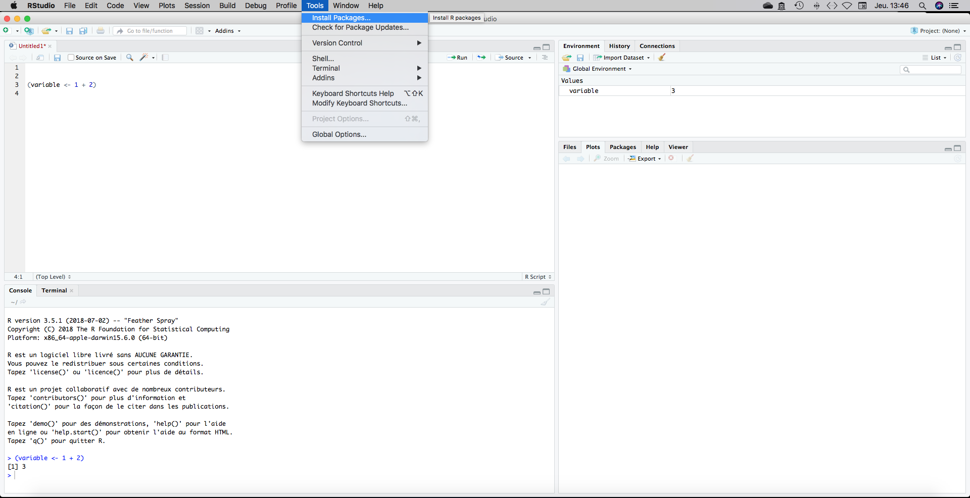
There is an autocompletion that will help you. We will need the following packages:
- ggplot2
- plyr
- dplyr
- reshape2
Install them one by one and load them by writing these line of code on your script.
library(ggplot2)
library(plyr)
library(dplyr)
library(reshape2)
How to load data?
Load your data by hand directly:
MyValues <- scan()Feed your “MyValues” variable with numbers and double press the Enter key when you are done. This can be an easy solution when you want to perfom a simple t.test for example.
A <- scan() #I loaded 10,15,14,26,51,24,22,41,56,57,41,23,25,20,30
B <-scan() #I loaded 80,78,98,56,25,36,54,87,89,69,58,95,85,84,70
t.test(A,B) #Compared A and B with a Student t.test##
## Welch Two Sample t-test
##
## data: A and B
## t = -5.9842, df = 25.31, p-value = 2.857e-06
## alternative hypothesis: true difference in means is not equal to 0
## 95 percent confidence interval:
## -54.56434 -26.63566
## sample estimates:
## mean of x mean of y
## 30.33333 70.93333wilcox.test(A,B) #Compared A and B with a Wilcoxon test (non-parametric)## Warning in wilcox.test.default(A, B): cannot compute exact p-value with ties##
## Wilcoxon rank sum test with continuity correction
##
## data: A and B
## W = 16, p-value = 6.799e-05
## alternative hypothesis: true location shift is not equal to 0But this is not going to be a solution when you have hundreds of values or more to load! I don’t even use this scan() function but it is good to know it is there.
Load your data in a variable as a vector.
A vector is a concatenation of several items, it can be numbers or letters. In R, letters have to be into "".
Note here that I used NA. NA = NonAvailable and is the standard value for blank values in R.
Time<-c(1,2,3,4,5,6)

Event=c("Yes","Yes","No","Yes","No",NA)
Load your data in a variable in a data.frame.
Several vectors of the same length can be concatenated into a data.frame. Here I am creating a data.frame called “dat” that contains two columns: “Time”" and “Event”.
(dat <- data.frame(Time=c(1,2,3,4,5,6) , Event=c("Yes","Yes","No","Yes","No",NA) ))## Time Event
## 1 1 Yes
## 2 2 Yes
## 3 3 No
## 4 4 Yes
## 5 5 No
## 6 6 <NA>Load your data by loading a file.
This is much more convenient when you have to load a lot of values.
There are a lot of possibility to do that. We will see here the basic read.table() function.
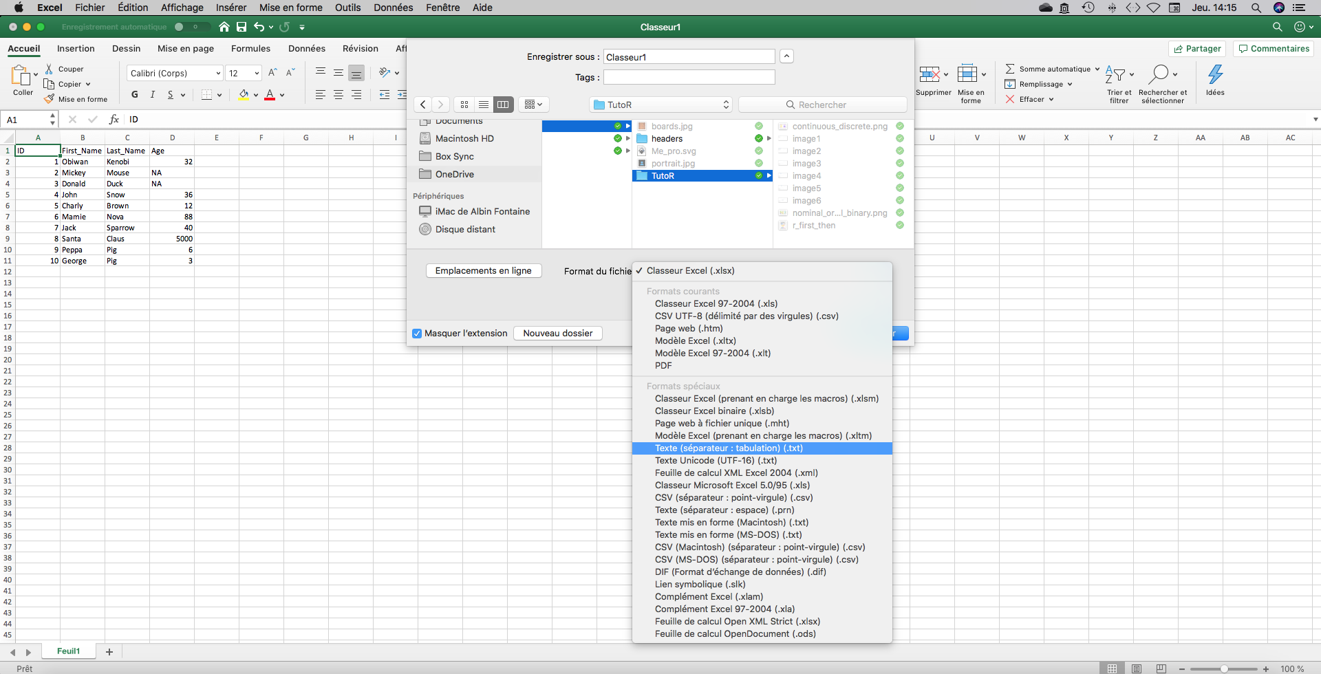
Before to do that, we have to open an Excel spreadsheet. Excel is a good spreadsheet program and I always used it to format my data input for R. There are important rules to follow:
- In the spreadsheet, my data are usually formated with individuals in lines and observations in columns. My first line is often used for colmun names.
- Blank (empty) cells in R are your enemies! Use ctrl-F to detect and replace them by “NA”.
- Make sure that you don’t use a same column name twice!
- Make sure that there is no spaces in your Excel cells!
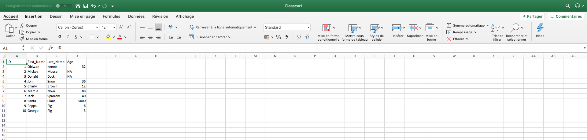
All of these are double checked? Then you can save your Excel spreadsheet in text (.txt) with tabular separation. Be aware that all colors or other nice topings you can have added in you Excel spreadsheet will be lost. There are useless anyway, R cannot read color or font informations. Every information has to be coded in a new column. Make sure that you used the same way to code for a value. For instance, R will see “Yes” and “yes” as two different things.
I often use .txt input files (with tabular separation) because Excel .csv have different separators in USA/UK version vs French version. It can be a nightmare when you share files with people outside France. But a read.csv() function is available.
Note: RStudio help you to find your file. Once you clic inside a "" press the tab key to have the autocompletion tool.
#my_data <- read.table("/img/TutoR/Classeur1.txt", header = TRUE) #for .txt input data

#my_data <- read.csv("path_to_data.csv", header = TRUE, sep=";") #for .csv (coma separated values) input data, you can change the separator, eg ","
By adding header= TRUE as an argument, I am specifying that the first line of my Excel spreadsheet will be used as column names.
Once it is done you can easily display the first lines of your data with the head(function)
#head(my_data)The 6 first rows are displayed by default, but you can control that:
#head(my_data, 10) #display the 10 first linesYou might have noticed that I am using the hashtag symbol ( #) in my code to add some text. The exact term is “to comment my code”. R will consider everything as commentary after a # and will not try to execute it.
The different type of data that you can handle
R can deal with numbers and text. By default, R will make a guess about the type of data you are giving it. You can have a glimpse of the data type with the str() function.
In R, a function always end by “()”. You can see the help for the function by typing ?function.name(). The help will then display on the “Help” tab on the bottom-right panel.
Here str() (structure) will tell you that the variable “my_data” is a data.frame with 4 variables (columns) and 10 observations per variable. It will also tells you how variables are treated:
#str(my_data)
#?str()
chr (=character). Type of data make with letters.
Factor. Factor data can be either number or letter but are treated as a “label”. By default a factor is just a label and R would not put a value on them. However, you can specifically order factor labels.
my_labels <- factor(c("mid","low", "high"))
my_labels
## [1] mid low high
## Levels: high low midstr(my_labels)## Factor w/ 3 levels "high","low","mid": 3 2 1my_labels_order <- factor(c("mid","low", "high"), levels=c("low", "mid", "high"))
my_labels_order## [1] mid low high
## Levels: low mid highstr(my_labels_order)## Factor w/ 3 levels "low","mid","high": 2 1 3int (integer). Numerical data with integer (continuous, no coma)
num Numerical data (continuous, with coma)
Numerical values can be contiunous or discrete. Allison Horst @allison_horst made a nice drawing to help you to distinguish between both.
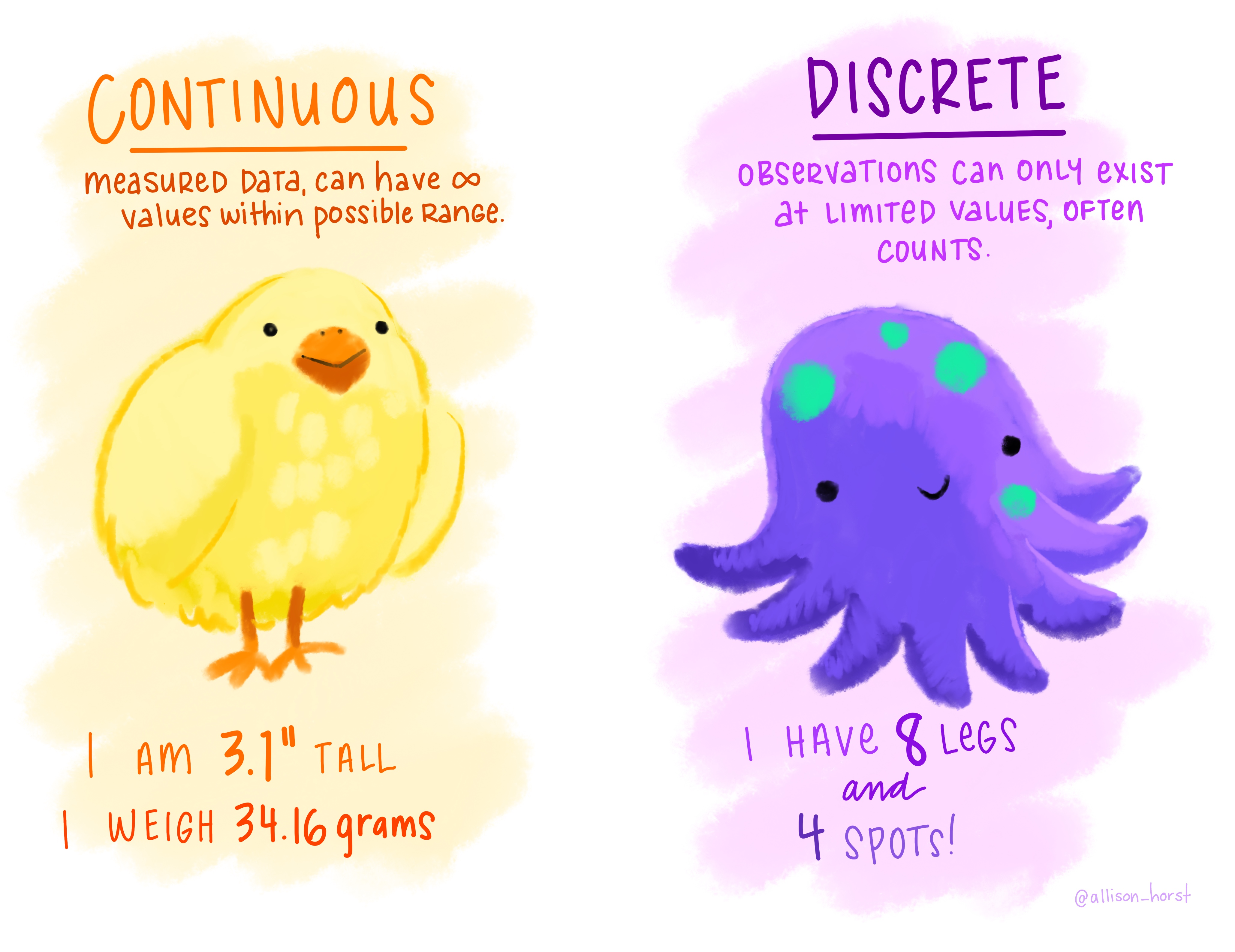 Image from https://github.com/allisonhorst/stats-illustrations
Another drawing to help you to distinguish between nominal, ordinal and binary data:
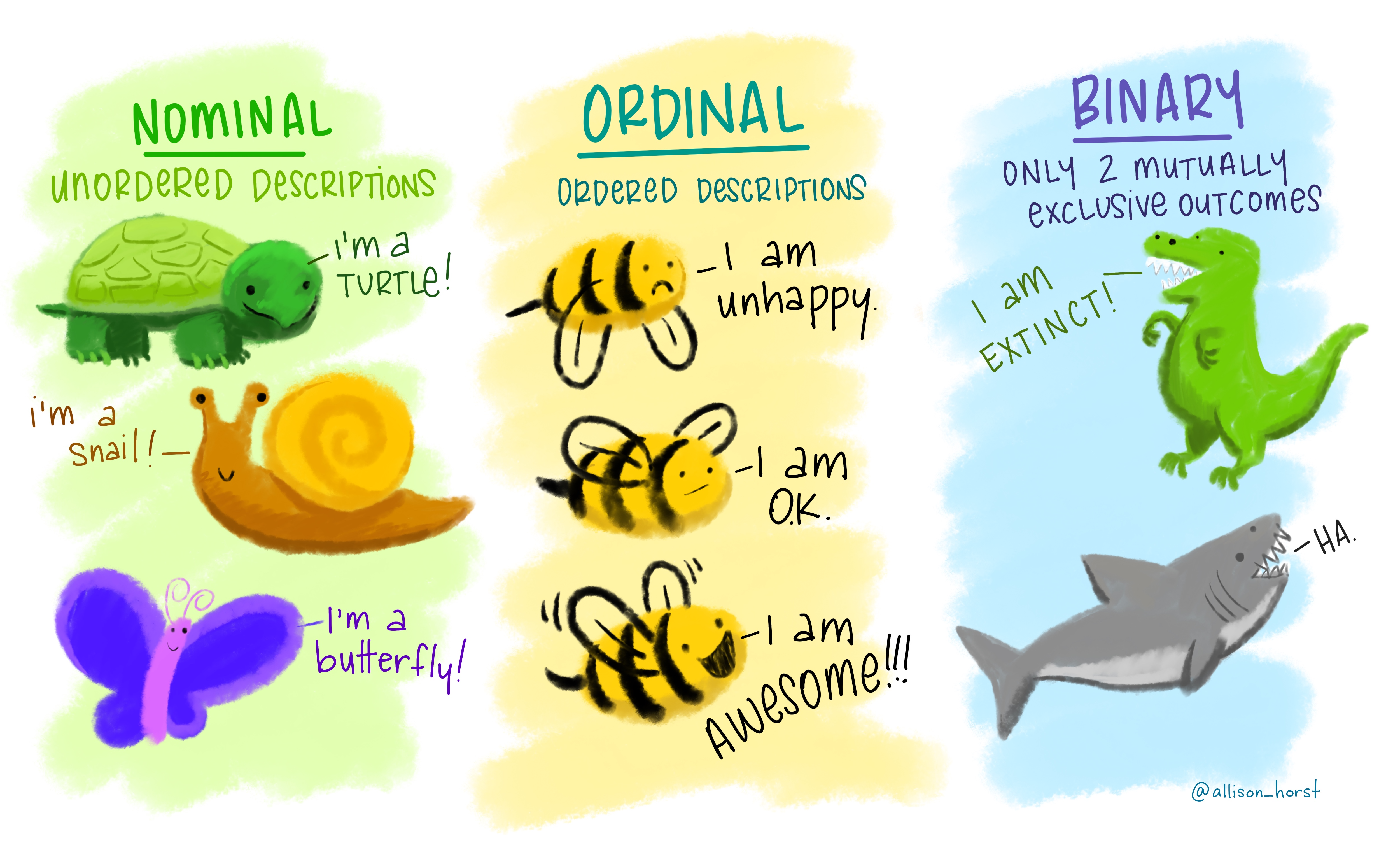 Image from https://github.com/allisonhorst/stats-illustrations
Data.frame manipulation
For the demo, we are going to use the “mtcars”" prebuilt R dataset.
We can first display the first rows, then the structure of the dataset:
head(mtcars)## mpg cyl disp hp drat wt qsec vs am gear carb
## Mazda RX4 21.0 6 160 110 3.90 2.620 16.46 0 1 4 4
## Mazda RX4 Wag 21.0 6 160 110 3.90 2.875 17.02 0 1 4 4
## Datsun 710 22.8 4 108 93 3.85 2.320 18.61 1 1 4 1
## Hornet 4 Drive 21.4 6 258 110 3.08 3.215 19.44 1 0 3 1
## Hornet Sportabout 18.7 8 360 175 3.15 3.440 17.02 0 0 3 2
## Valiant 18.1 6 225 105 2.76 3.460 20.22 1 0 3 1str(mtcars)## 'data.frame': 32 obs. of 11 variables:
## $ mpg : num 21 21 22.8 21.4 18.7 18.1 14.3 24.4 22.8 19.2 ...
## $ cyl : num 6 6 4 6 8 6 8 4 4 6 ...
## $ disp: num 160 160 108 258 360 ...
## $ hp : num 110 110 93 110 175 105 245 62 95 123 ...
## $ drat: num 3.9 3.9 3.85 3.08 3.15 2.76 3.21 3.69 3.92 3.92 ...
## $ wt : num 2.62 2.88 2.32 3.21 3.44 ...
## $ qsec: num 16.5 17 18.6 19.4 17 ...
## $ vs : num 0 0 1 1 0 1 0 1 1 1 ...
## $ am : num 1 1 1 0 0 0 0 0 0 0 ...
## $ gear: num 4 4 4 3 3 3 3 4 4 4 ...
## $ carb: num 4 4 1 1 2 1 4 2 2 4 ...All variable are numercial. This is a data.frame.
Dimension of the data.set:
dim(mtcars)## [1] 32 1132 lines, 11 columns
Row names, and column names
row.names(mtcars)## [1] "Mazda RX4" "Mazda RX4 Wag" "Datsun 710"
## [4] "Hornet 4 Drive" "Hornet Sportabout" "Valiant"
## [7] "Duster 360" "Merc 240D" "Merc 230"
## [10] "Merc 280" "Merc 280C" "Merc 450SE"
## [13] "Merc 450SL" "Merc 450SLC" "Cadillac Fleetwood"
## [16] "Lincoln Continental" "Chrysler Imperial" "Fiat 128"
## [19] "Honda Civic" "Toyota Corolla" "Toyota Corona"
## [22] "Dodge Challenger" "AMC Javelin" "Camaro Z28"
## [25] "Pontiac Firebird" "Fiat X1-9" "Porsche 914-2"
## [28] "Lotus Europa" "Ford Pantera L" "Ferrari Dino"
## [31] "Maserati Bora" "Volvo 142E"colnames(mtcars)## [1] "mpg" "cyl" "disp" "hp" "drat" "wt" "qsec" "vs" "am" "gear"
## [11] "carb"Select lines and columns
A data.frame column can be selected via the $ symbol. If I want to select the “mpg” column:
mtcars$mpg## [1] 21.0 21.0 22.8 21.4 18.7 18.1 14.3 24.4 22.8 19.2 17.8 16.4 17.3 15.2 10.4
## [16] 10.4 14.7 32.4 30.4 33.9 21.5 15.5 15.2 13.3 19.2 27.3 26.0 30.4 15.8 19.7
## [31] 15.0 21.4I can also use the very convenient: “[,]” symbol (on Mac press alt+shift+bracket to have []). With the [,], the coma “,” separate the lines from the columns.
So if I want to select the first row:
mtcars[1,]## mpg cyl disp hp drat wt qsec vs am gear carb
## Mazda RX4 21 6 160 110 3.9 2.62 16.46 0 1 4 4Second column
mtcars[,2]## [1] 6 6 4 6 8 6 8 4 4 6 6 8 8 8 8 8 8 4 4 4 4 8 8 8 8 4 4 4 8 6 8 4Also, we can directly specify a column name
mtcars[,"mpg"]## [1] 21.0 21.0 22.8 21.4 18.7 18.1 14.3 24.4 22.8 19.2 17.8 16.4 17.3 15.2 10.4
## [16] 10.4 14.7 32.4 30.4 33.9 21.5 15.5 15.2 13.3 19.2 27.3 26.0 30.4 15.8 19.7
## [31] 15.0 21.4First row and column 1 to 4
mtcars[1,c(1,2,3,4)]## mpg cyl disp hp
## Mazda RX4 21 6 160 110#or
mtcars[1,c(1:4)]## mpg cyl disp hp
## Mazda RX4 21 6 160 110You probably grasp it. The R language is evolving fast. I first used the core R language and discovered the Tidyverse on the late. We will see later what is the Tidyverse. It is another way to code that make data manipulation easier. But one step at a time.
Making nice charts with ggplot2
Ok, it is time to built our first plot!
We will first call the ggplot function like this
p <- ggplot(data=mtcars,aes(x=cyl,y=mpg))Here, I specified my data variable (the mtcars data.frame) and an aesthetic (aes). I specified the column names of the data.frame that have to be treated as x and y. I treated the “cyl” values as factors.
Now we have to specify a plot layer. I am adding a new layer to the plot like this:
p <- ggplot(data=mtcars,aes(x=factor(cyl),y=mpg))
p <- p + geom_boxplot()
p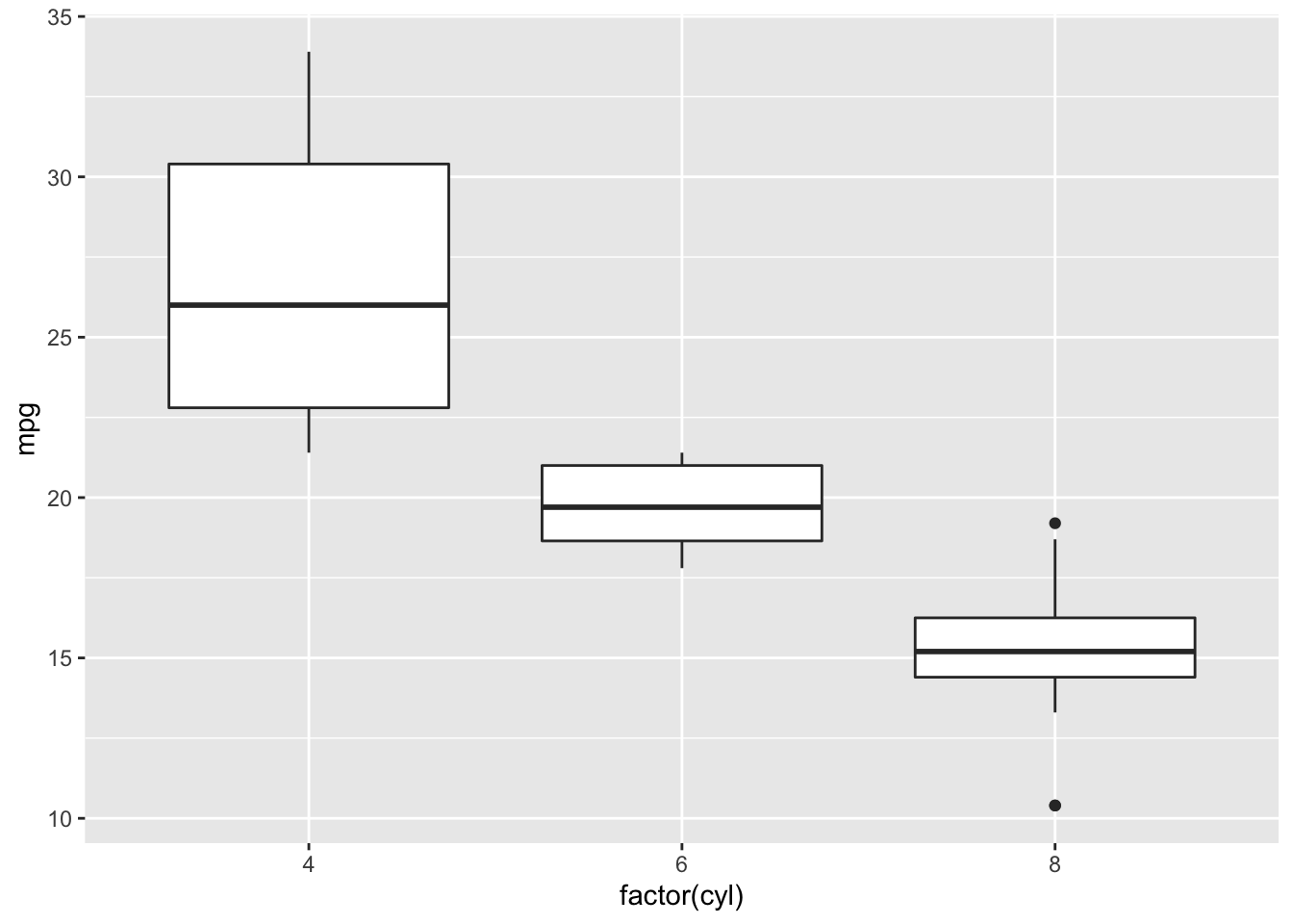
You first graph should have appeared on the “Plots” pannel!!!
Here is shown the fuel consumption in miles per gallon according to the number of cylinders. I am used to the liter per 100 km value, the lesser is the better in term of fuel consumption. Mpg is the opposite, higher values mean less fuel consumption because you can drive more miles for a gallon. That totally suits to the US I guess.
We are going to make it nicer by adding new layers to the plot.
require("grid") #same as library() function,it is used to load the grid package that can add some space (margins) around your plot.## Le chargement a nécessité le package : gridp <- ggplot(data=mtcars,aes(x=factor(cyl),y=mpg))
p <- p + geom_boxplot(color="red", fill="lightblue")
p <- p + theme_light(base_size =20) #add a nice theme, you can change the theme easily:eg. theme_classic(), theme_dark(), theme_minimal(). Base_size is the base text size.
p <- p + xlab("Cylinders") + ylab("Miles per Gallon") #add x and y labels
p <- p + theme(plot.margin = unit(c(2,2,2,2), "lines")) #add margins around the plot
p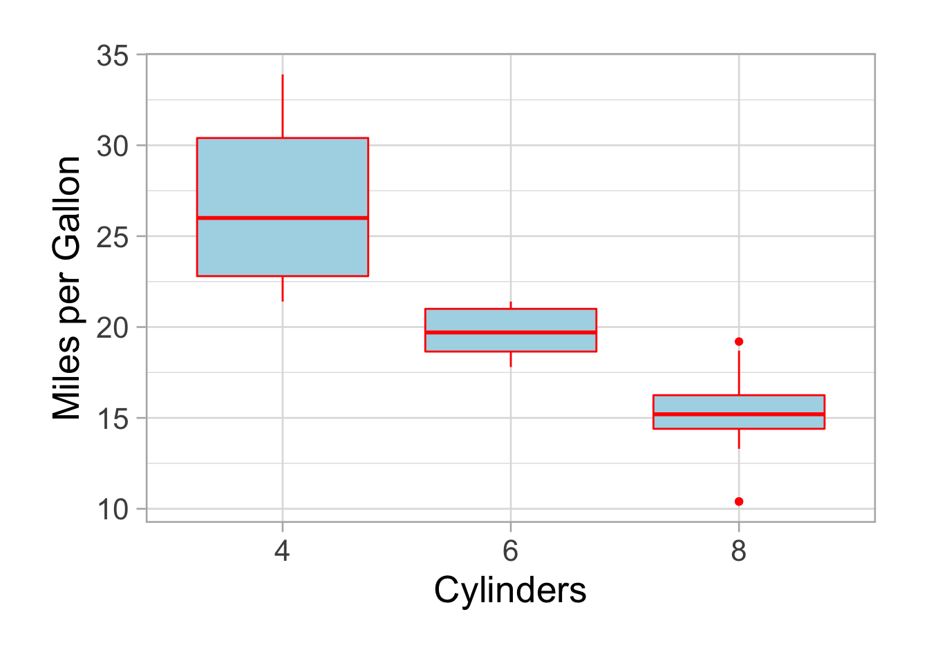
Much better. Colors sucks but it was to show you the differences between color (the stroke) and the fill.
Do you want to flip it:
p <- p + coord_flip()
p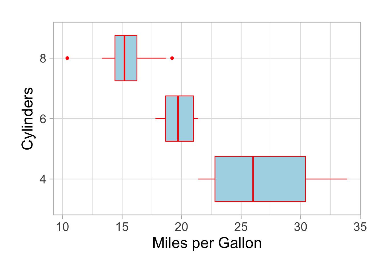
We have seen the geom_boxplot(), but there are so many possibilities.
require("grid") #same as library() function,it is used to load the grid package that can add some space (margins) around your plot.
p <- ggplot(data=mtcars,aes(x=wt,y=mpg))
p <- p + geom_point(color="red", size=3)
p <- p + theme_light(base_size =20) #add a nice theme, you can change the theme easily:eg. theme_classic(), theme_dark(), theme_minimal(). Base_size is the base text size.
p <- p + xlab("Weight (x 1000lbs)") + ylab("Miles per Gallon") #add x and y labels
p <- p + theme(plot.margin = unit(c(2,2,2,2), "lines")) #add margins around the plot
p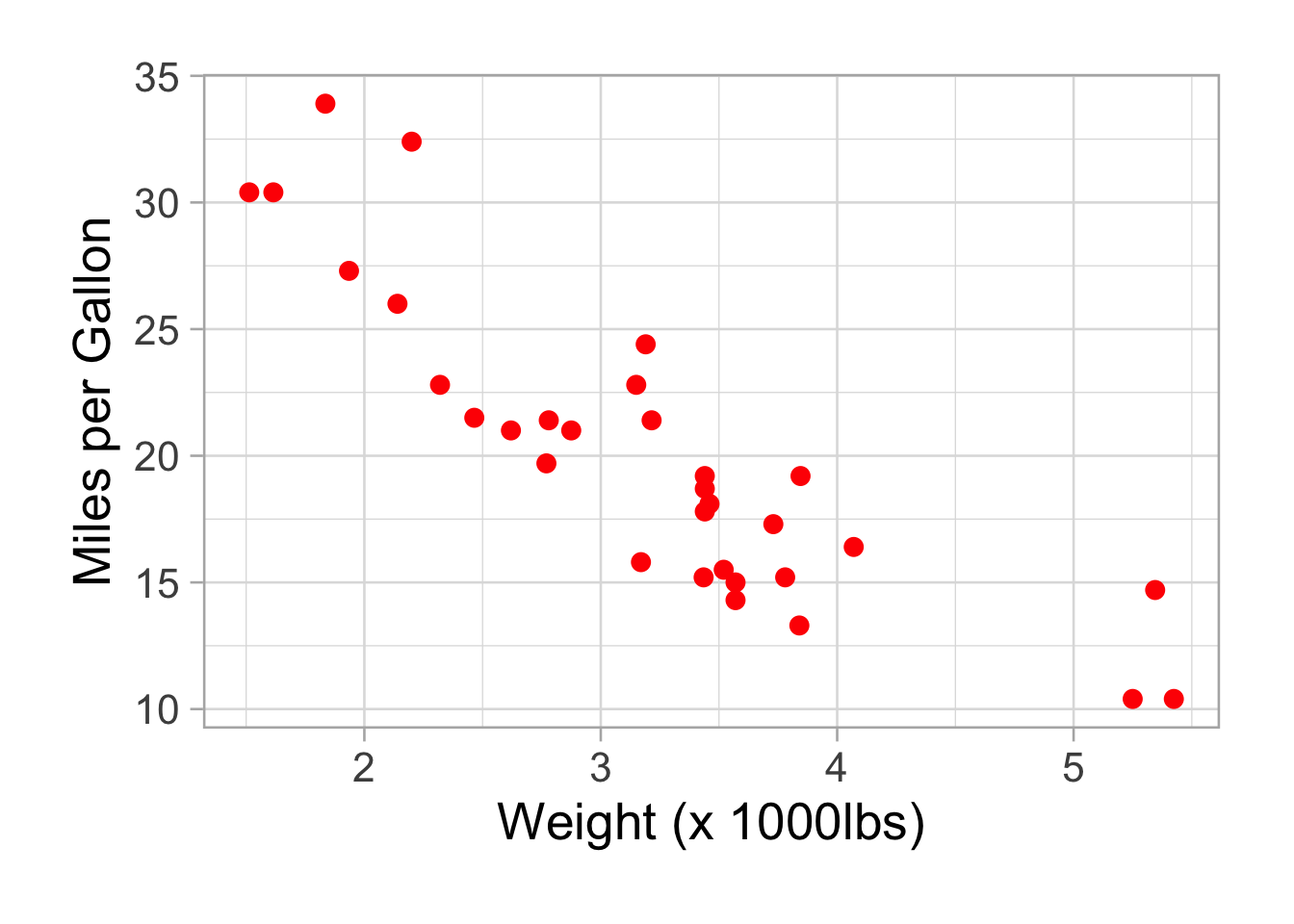
Add a regression line:
p <- p + geom_smooth(method = "lm")
p
## `geom_smooth()` using formula 'y ~ x'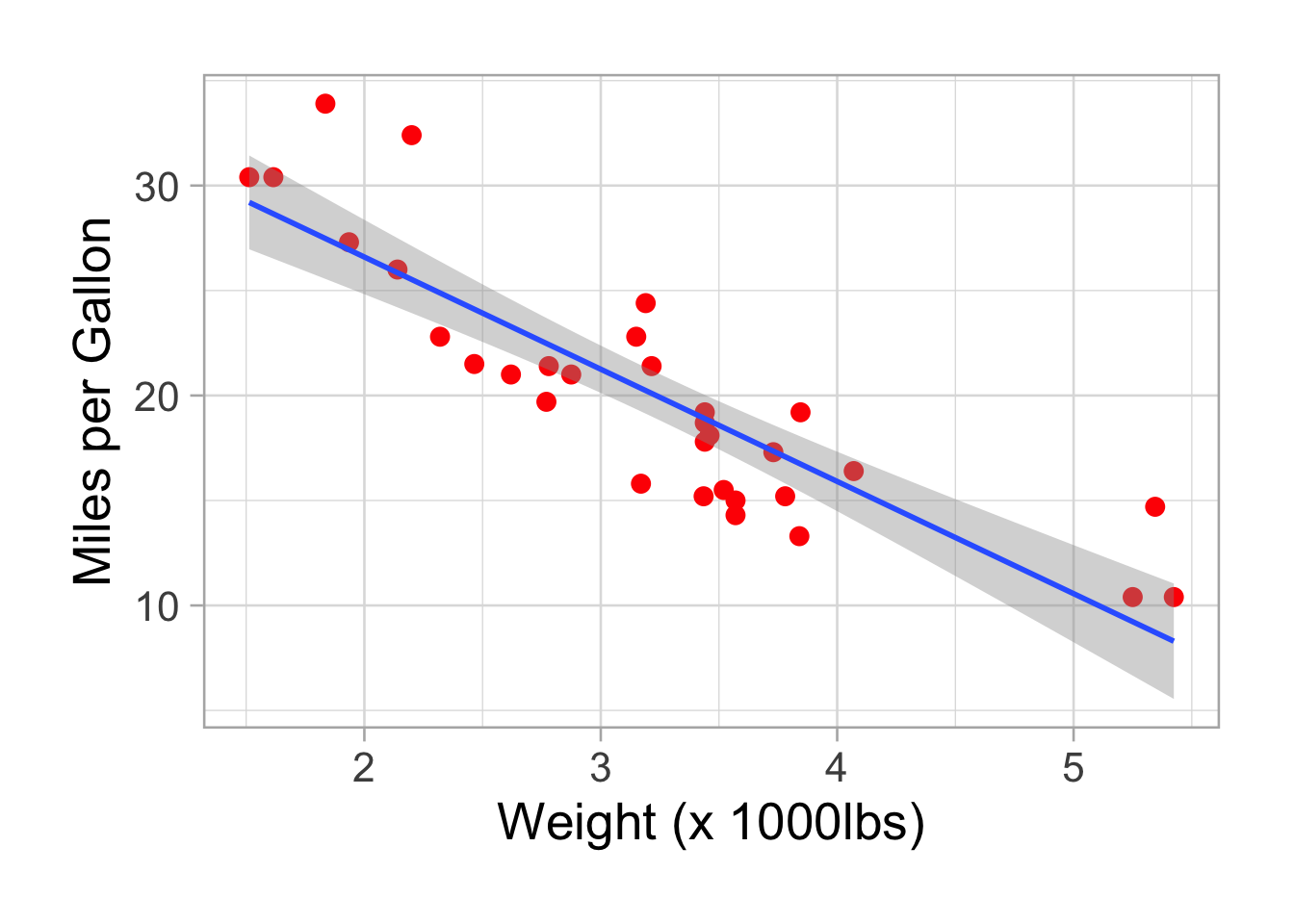
There is a nice negative correlation between fuel consumption (mpg) and car weight. Don’t be mislead once again, heavier cars burn more fuel, they cover less distances with one gallon.
We can add colors according to another variable. You have to add a grouping variable in the aes(), here the number of cylinders.
require("grid")
p <- ggplot(data=mtcars,aes(x=wt,y=mpg, col=factor(cyl))) #I add the col inside the aesthetic
p <- p + geom_point(size=3)
p <- p + theme_light(base_size =20)
p <- p + labs(x="Weight (x 1000lbs)", y="Miles per Gallon", colour="Number of\n Cylinders")
p <- p + theme(plot.margin = unit(c(2,2,2,2), "lines"))
p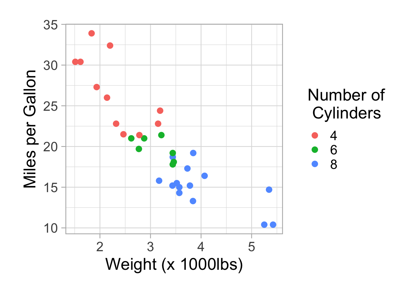
A legend appears. We can remove it with theme(legend.position = “none”).
Facetting.
p <- p + facet_wrap(~factor(cyl))
p <- p + theme(legend.position = "none")
p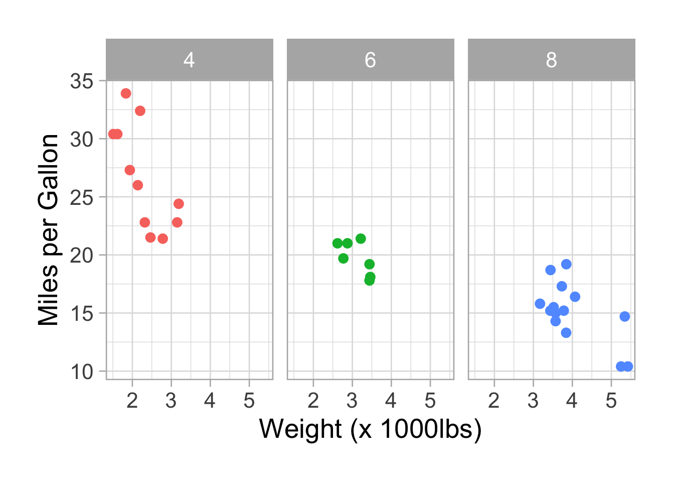
We can add the “free_x” option to free the x axis:
p <- p + facet_wrap(~factor(cyl), scales = "free_x")
p <- p + theme(legend.position = "none")
p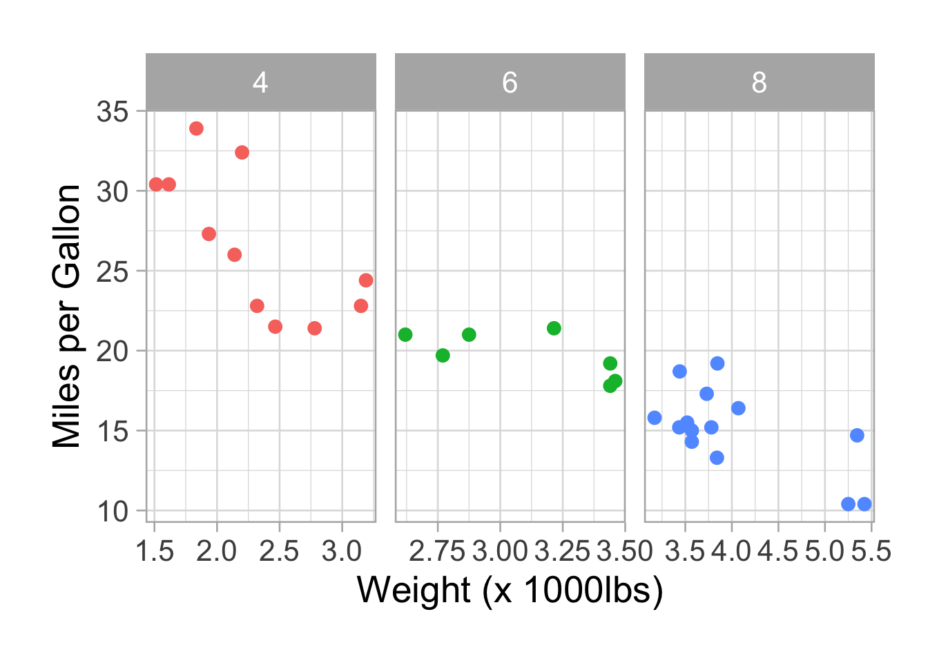
The ggpubr package
We will use the ggpubr package developed by Alboukadel Kassambara (http://www.alboukadel.com). I strongly recommend you to visit his website and have a look to all the tools his has developed. Factoextra, surviminer and ggpubr are all in my top 10 packages that I am using.
To install:
if(!require(devtools)) install.packages(“devtools”) devtools::install_github(“kassambara/ggpubr”)
We will continue to use the same dataset: mtcars
We will try to address the question: Is there a horsepower difference between cars with 3,4 and 5 gears? Lets install the (i) tidyverse and (ii) explore packages first.
The explore function is convenient to have a quick look at your data:
library(tidyverse)## ── Attaching packages ─────────────────────────────────────── tidyverse 1.3.1 ──## ✓ tibble 3.1.5 ✓ purrr 0.3.4
## ✓ tidyr 1.1.4 ✓ stringr 1.4.0
## ✓ readr 2.0.1 ✓ forcats 0.5.1## ── Conflicts ────────────────────────────────────────── tidyverse_conflicts() ──
## x dplyr::arrange() masks plyr::arrange()
## x purrr::compact() masks plyr::compact()
## x dplyr::count() masks plyr::count()
## x dplyr::failwith() masks plyr::failwith()
## x dplyr::filter() masks stats::filter()
## x dplyr::id() masks plyr::id()
## x dplyr::lag() masks stats::lag()
## x dplyr::mutate() masks plyr::mutate()
## x dplyr::rename() masks plyr::rename()
## x dplyr::summarise() masks plyr::summarise()
## x dplyr::summarize() masks plyr::summarize()library(explore)
mtcars %>% explore(var= hp, target = gear)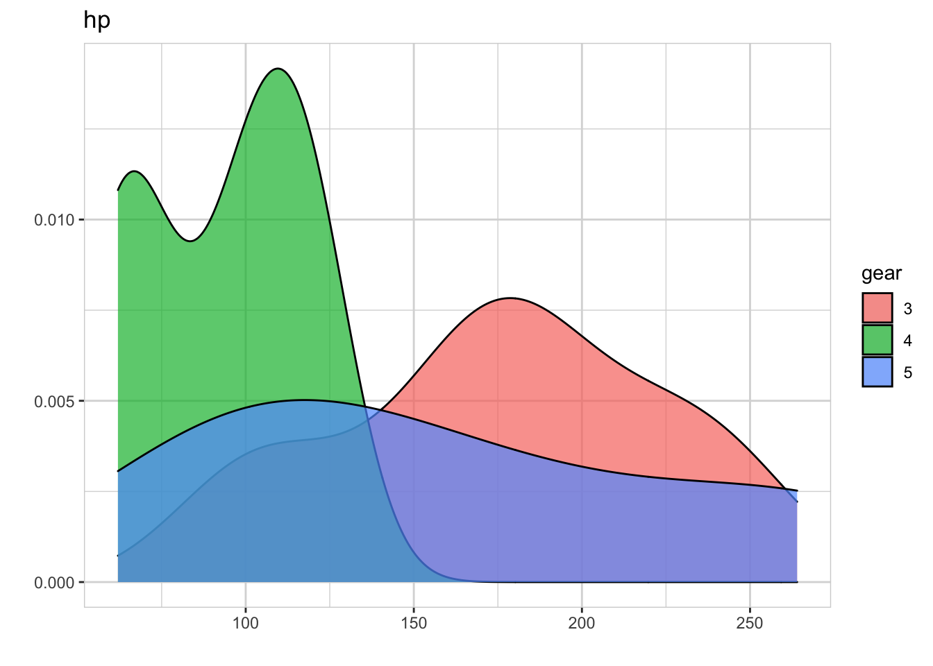
Horsepower looks different between cars with 3 and 4 gears. We now make all pairwise comparisons with only one line of code
library(ggpubr)##
## Attachement du package : 'ggpubr'## The following object is masked from 'package:plyr':
##
## mutate(A <- compare_means(hp ~ gear, data = mtcars, method = "t.test", p.adjust.method="bonferroni"))## # A tibble: 3 × 8
## .y. group1 group2 p p.adj p.format p.signif method
## <chr> <chr> <chr> <dbl> <dbl> <chr> <chr> <chr>
## 1 hp 4 3 0.00000441 0.000013 4.4e-06 **** T-test
## 2 hp 4 5 0.0817 0.25 0.082 ns T-test
## 3 hp 3 5 0.701 1 0.701 ns T-test#You can use a nonparametric method too by replacing the method by method = "wilcox.test"We can see that horsepower is significantly different between cars with 3 and 4 gears (p = 0.000184). We can easily plot with this code:
#First define the significant comparisons:
my_comparisons <- list( c("4", "3"))

p <- ggboxplot(mtcars, x = "gear", y = "hp", fill = "gear", palette = "jco") +
  stat_compare_means(comparisons = my_comparisons, method="t.test")+ # Add pairwise comparisons p-value
 stat_compare_means(label.y = 8) + theme(legend.position = "bottom", legend.box = "horizontal")    # Add global p-value
p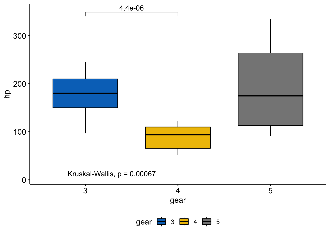
#ggsave("Plotname.pdf", p, width = 9,height = 7 )More to come soon.
Albin Fontaine
Researcher
My main research interests include vector-borne diseases surveillance, interaction dynamics between mosquito-borne pathogens and their hosts, and quantitative genetics applied to mosquito-viruses interactions.