The Reed and Muench method to estimate a median lethal dose (LD50) implemented in R

A endpoint dilution assay quantifies the amount of a test substance (ie. drug, toxin, pathogen, etc…) that produces an effect of interest in a given proportion of test units (ie. mice, cells, etc…). Endpoint dilution assays require to submit batches of several test units to different dose dilutions and record the output. Reed and Muench, 1938, have designed a well known method to calculate the median lethal dose (LD50) based on endpoint dilution assay outputs http://aje.oxfordjournals.org/content/27/3/493.full.pdf+html.

This code was used for the paper “Exchanges of genomic domains between poliovirus and other cocirculating species C enteroviruses reveal a high degree of plasticity.” (https://www.ncbi.nlm.nih.gov/pubmed/27958320).

We will need these packages:

-library(plyr)
-library(dplyr)
-library(ggplot2)
-library(FSA)
-library(grid)
-library(reshape2)

#Uncomment (remove the # before lines) these lines to install packages. This has to be done only once. Comment the line again when it has been done.

#install.packages("plyr")
#install.packages("dplyr")
#install.packages("ggplot2")
#install.packages("FSA")
#install.packages("grid")
#install.packages("reshape2")

library(plyr)
library(dplyr)
library(ggplot2)
library(FSA)
library(grid)
library(reshape2)

Graphical representation and LD50 estimation

One asset of this method is that we can easily represent graphically the results. We will here plot the data and find a LD50 estimate “by eye”.

data.plot <- melt(data2, .(Log10_virus_dilution, Inoculated_mice, Death, Alive, Cumulative_Total, Percentage_Death ))


p0 <- ggplot()
p0 <- p0 + geom_line(data=data.plot, aes(x=Log10_virus_dilution, y=value, colour=variable), size=1.5)
p0 <- p0 + theme_bw(base_size =20) + scale_x_reverse()
p0 <- p0 + ylab("Nbr of mice") + xlab(label="Log(Dose)")
p0 <- p0 + ggtitle("") + scale_color_manual(values = c("dodgerblue3", "deeppink2"))
#p0 <- p0 + theme(legend.position = "none")
p0 <- p0 + theme(axis.title.x=element_text(size=20, color="black", vjust=-1), axis.title.y=element_text(size=20, color="black", vjust=1, margin=margin(0,20,0,0)))
p0 <- p0 + theme(plot.margin = unit(c(2,2,2,2), "lines"))
print(p0)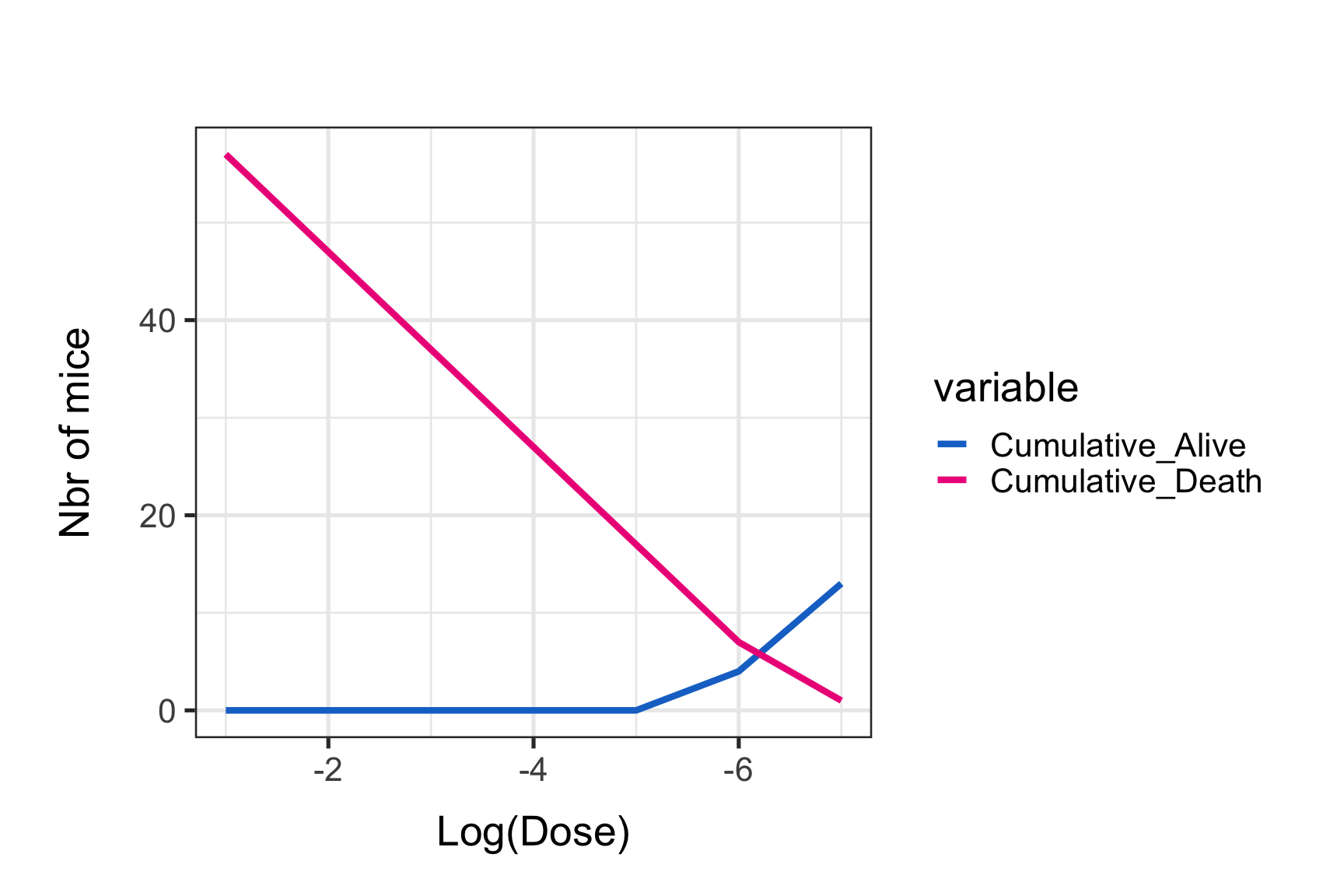

We can see that the intersection point is around 6 for the log10(dose) value by eyes.

But we want something more acurate.

These lines are just segments put ends to ends. Each segment can be defined by a x1, x2 y1 and y2. It is thus possible to find their mathematical equations. We are first going to select segments from the two curves that cross each other. Then we define their equations: Y1= slope*X + intercept. Then put Y1=Y2 to find the common X value.

x1=data2$Cumulative_Alive
x2=data2$Cumulative_Death
# Find points where x1 is above x2.
above<-x1>x2
# Points intersect when above=TRUE
intersect.points<-which(diff(above)!=0)
# Find the slopes for each line segment.
x1.slopes<- (x1[intersect.points]-x1[intersect.points+1]) / (data2$Log10_virus_dilution[intersect.points]-data2$Log10_virus_dilution[intersect.points+1])
x2.slopes<- (x2[intersect.points]-x2[intersect.points+1]) / (data2$Log10_virus_dilution[intersect.points]-data2$Log10_virus_dilution[intersect.points+1])

# Find the intersection for each segment.
x.points<-data2$Log10_virus_dilution[intersect.points] + ((x2[intersect.points] - x1[intersect.points]) / (x1.slopes-x2.slopes))
y.points<-x1[intersect.points] + (x1.slopes*(x.points-data2$Log10_virus_dilution[intersect.points]))
# Plot.

p0 <- p0 + geom_vline(xintercept = x.points, colour="orange", linetype = "longdash")
print(p0)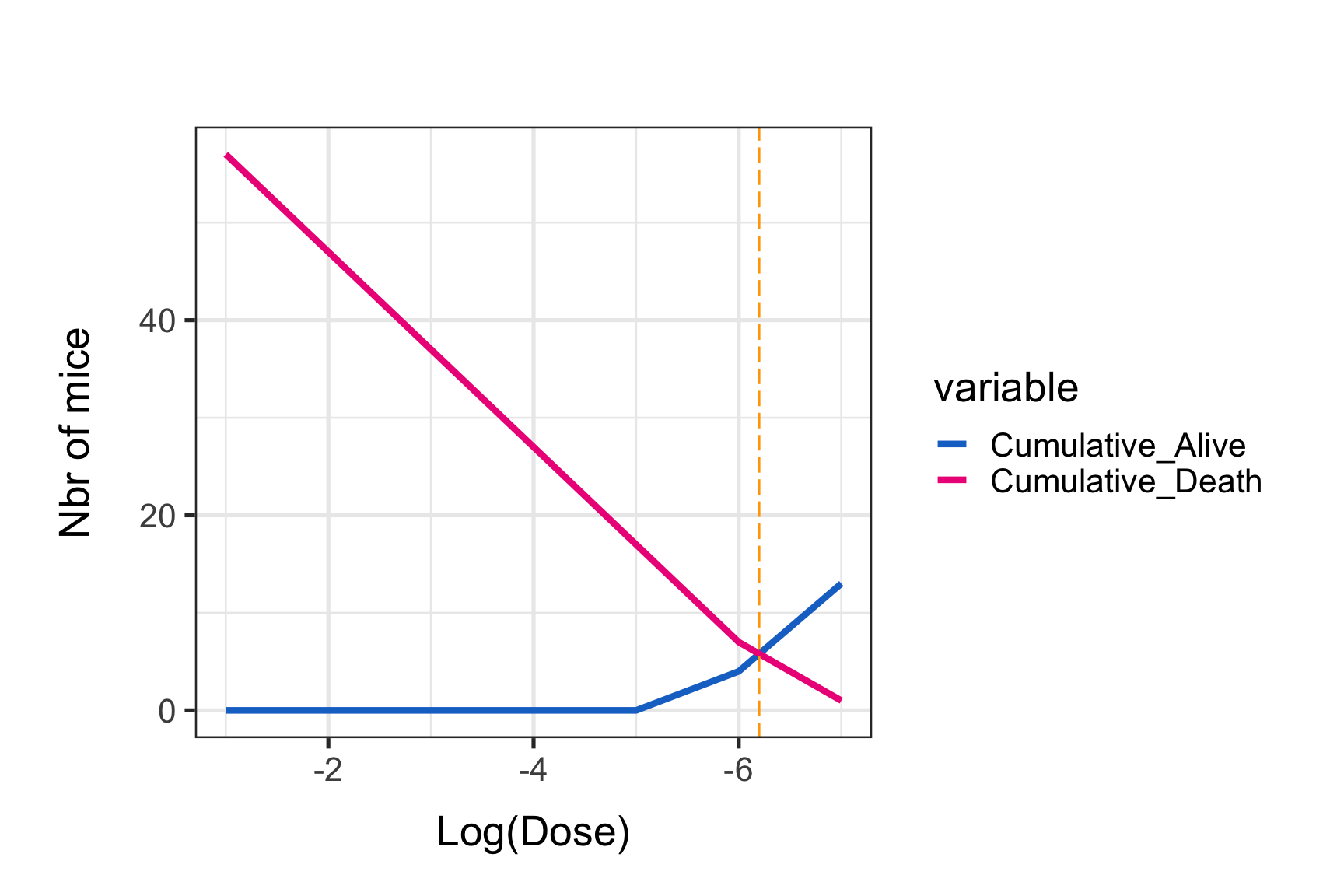

Notice the orange vertical line at the intersection point. The graphical estimate of the LD50 is:

paste("log(10) 50% end-point dilution :", x.points)

## [1] "log(10) 50% end-point dilution : -6.2"

paste("50% end-point dilution:", formatC((10^x.points), format = "e", digits = 2))

## [1] "50% end-point dilution: 6.31e-07"

paste("The virus titer (dose that kills 50% of mice, DL50) is:", formatC((10^(abs(x.points))), format = "e", digits = 2),"LD50/mL")

## [1] "The virus titer (dose that kills 50% of mice, DL50) is: 1.58e+06 LD50/mL"

LD50 estimation using a formula

It is possible to estimate LD50 using a formula. I was also inspired from the Muthannan Andavar Ramakrishnan paper (https://www.ncbi.nlm.nih.gov/pmc/articles/PMC4861875/).

We have to calculate what is called the “difference of logarithms” first:

Difference of logarithms = [(mortality at dilution next above 50%)-50%]/[(mortality at dilution next above 50%)-(mortality at dilution next below 50%)].

Then we can calculate the log10 50% end point dilution:

log10 50% end point dilution = log10 of dilution showing a mortality next above 50% - (difference of logarithms × logarithm of dilution factor).

mortality_at_dilution_next_above_50perc <- min(data2[which(data2$Percentage_Death > 50),"Percentage_Death"])
mortality_at_dilution_next_below_50perc <- max(data2[which(data2$Percentage_Death < 50),"Percentage_Death"])

Difference_of_logarithms = (mortality_at_dilution_next_above_50perc-50)/(mortality_at_dilution_next_above_50perc - mortality_at_dilution_next_below_50perc)

L10EPD <- min(data2[which(data2$Percentage_Death > 50),"Log10_virus_dilution"]) - (Difference_of_logarithms * 1)

paste("log(10) 50% end-point dilution :", L10EPD)

## [1] "log(10) 50% end-point dilution : -6.24137931034483"

paste("50% end-point dilution:", formatC((10^L10EPD), format = "e", digits = 2))

## [1] "50% end-point dilution: 5.74e-07"

paste("The virus titer (dose that kills 50% of mice, DL50) is:", formatC((10^(abs(L10EPD))), format = "e", digits = 2),"LD50/mL")

## [1] "The virus titer (dose that kills 50% of mice, DL50) is: 1.74e+06 LD50/mL"

Both methods give similar estimates of the LD50!